Linjediagram

Introduktion till datavisualisering med ggplot2

Rick Scavetta

Founder, Scavetta Academy

Vanliga diagramtyper

Diagramtyp	Möjliga geoms
Punktdiagram	points, jitter, abline, smooth, count
Stapeldiagram	histogram, bar, col, errorbar
Linjediagram	line, path

Beaver

str(beaver)

'data.frame':    101 obs. of  3 variables:
 $ time  : POSIXct, format: "2000-01-01 09:30:00" "2000-01-01 09:40:00" "2000-01-01 09:50:00" ...
 $ temp  : num  36.6 36.7 36.9 37.1 37.2 ...
 $ active: Factor w/ 2 levels "0","1": 1 1 1 1 1 1 1 1 1 1 ...

Beaver

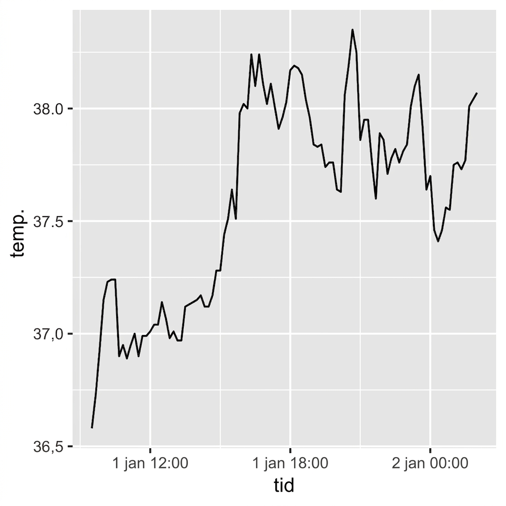
ggplot(beaver, aes(x = time, y = temp)) +
  geom_line()

Beaver

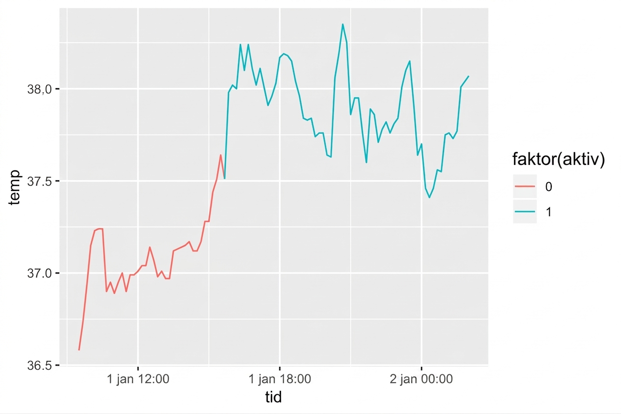
ggplot(beaver, aes(x = time, y = temp, 
                   color = factor(active))
                   ) +
  geom_line()

Datamängden fish catch

str(fish)

'data.frame':    427 obs. of  3 variables:
 $ Species: Factor w/ 7 levels "Pink","Chum",..: 1 2 3 4 5 6 7 1 2 3 ...
 $ Year   : int  1950 1950 1950 1950 1950 1950 1950 1951 1951 1951 ...
 $ Capture: int  100600 139300 64100 30500 0 23200 10800 259000 155900 51200 ...

Estetiken linetype

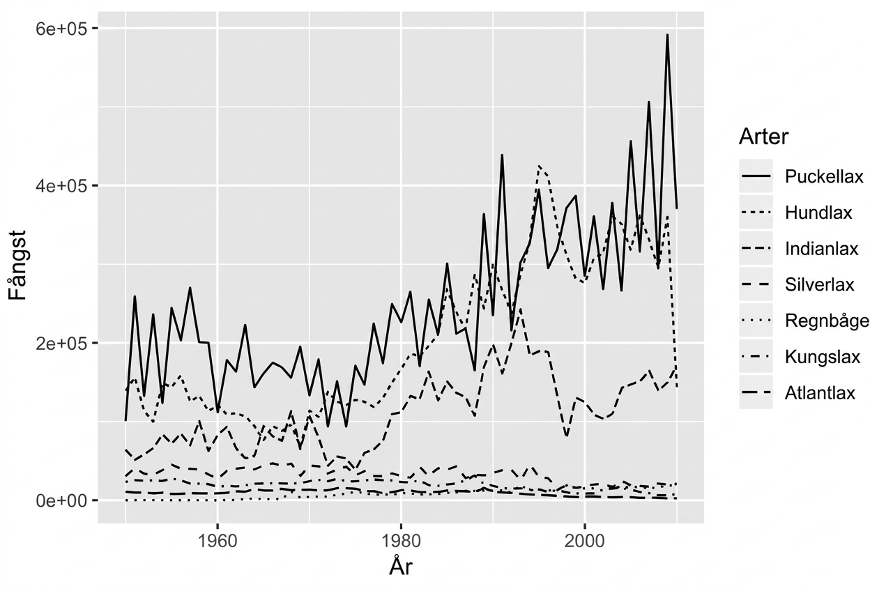
ggplot(fish, aes(x = Year, 
                 y = Capture, 
                 linetype = Species)) + 
  geom_line()

Estetiken size

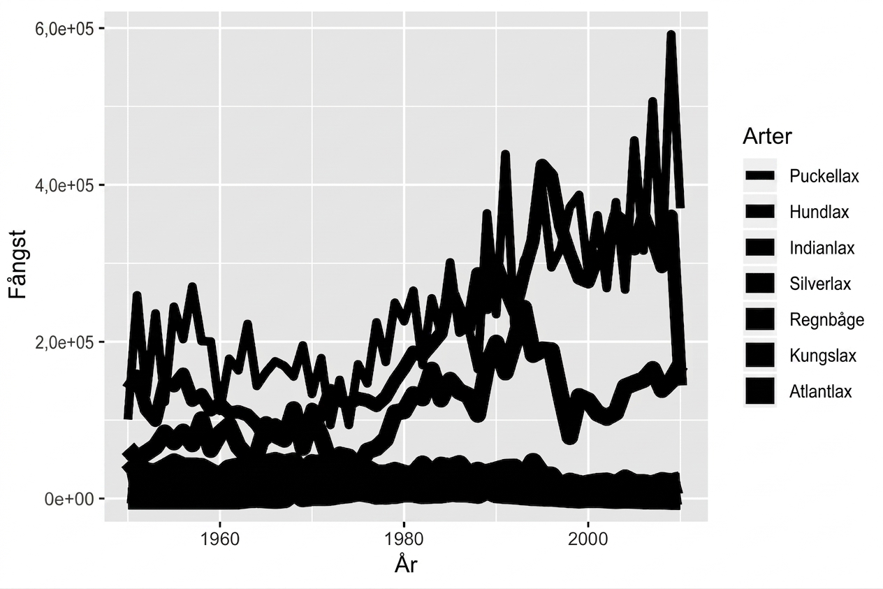
ggplot(fish, aes(x = Year, 
                 y = Capture, 
                 size = Species)) + 
  geom_line()

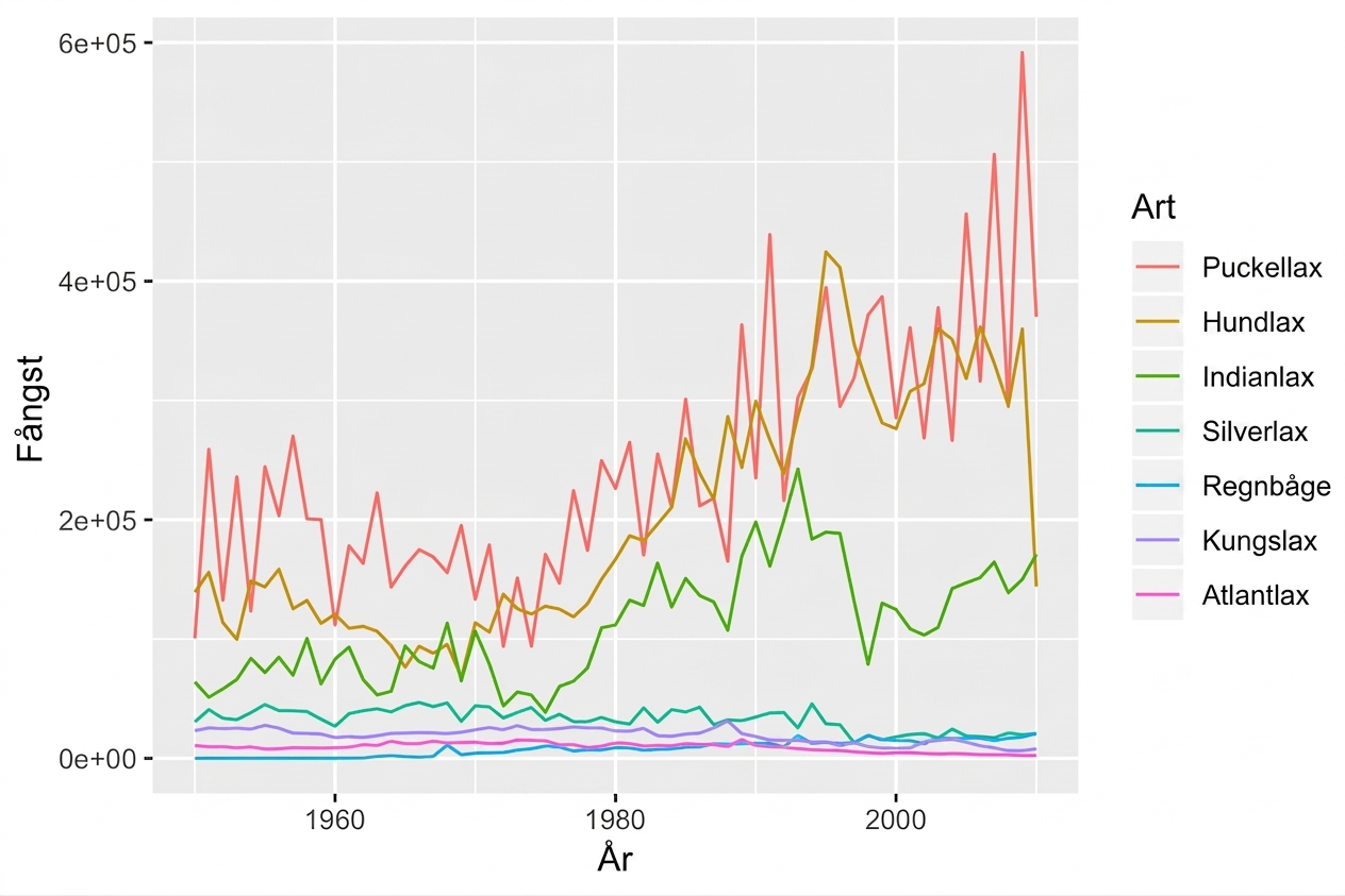
Estetiken color

ggplot(fish, aes(x = Year, 
                 y = Capture, 
                 color = Species)) + 
  geom_line()

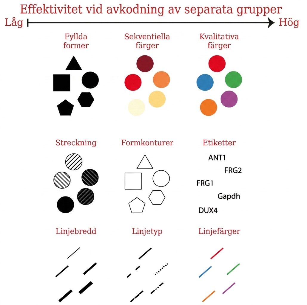
Estetik för kategoriska variabler

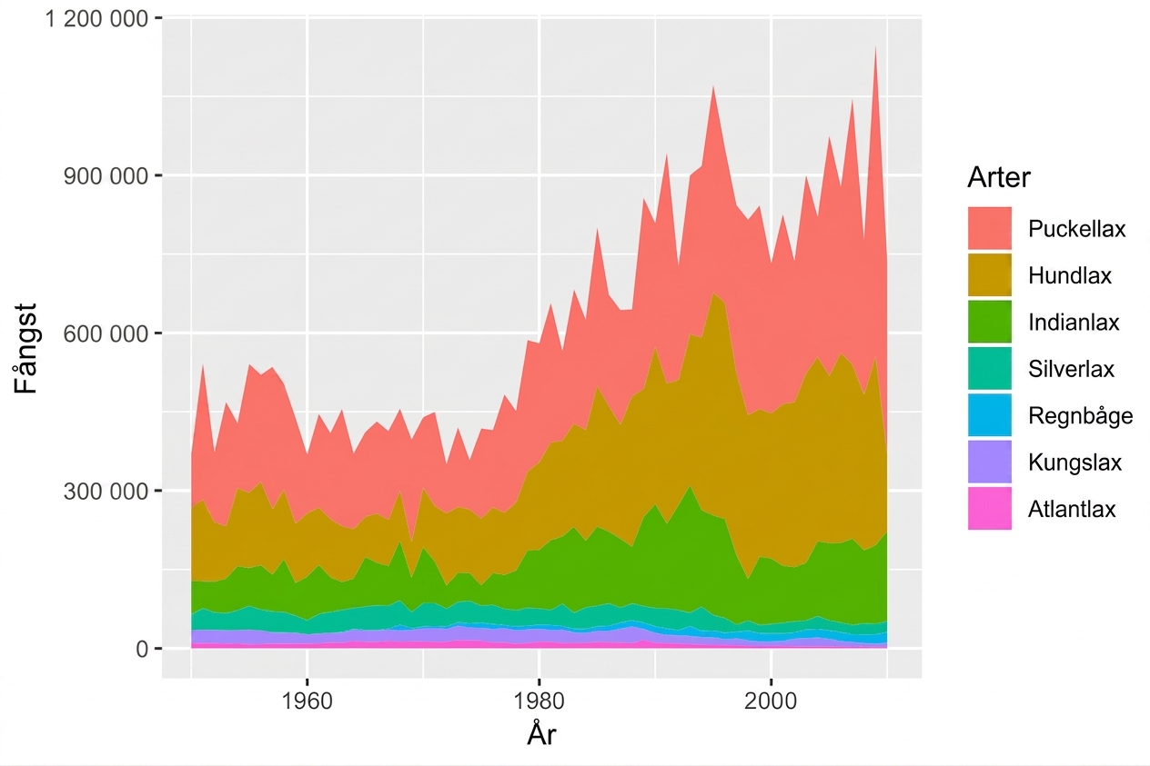
Estetiken fill med geom_area()

ggplot(fish, aes(x = Year, 
                 y = Capture, 
                 fill = Species)) + 
  geom_area()

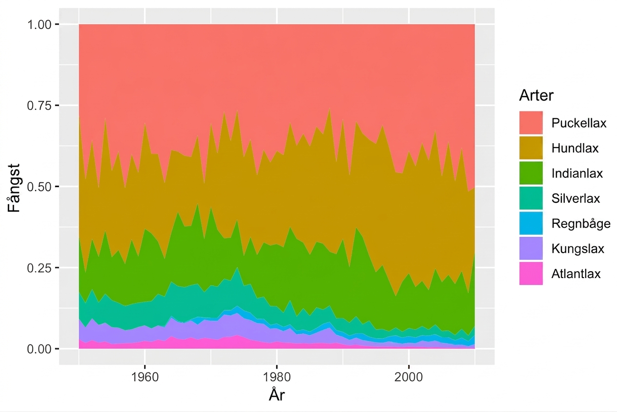
Använda position = "fill"

ggplot(fish, aes(x = Year, 
                 y = Capture, 
                 fill = Species)) + 
  geom_area(position = "fill")

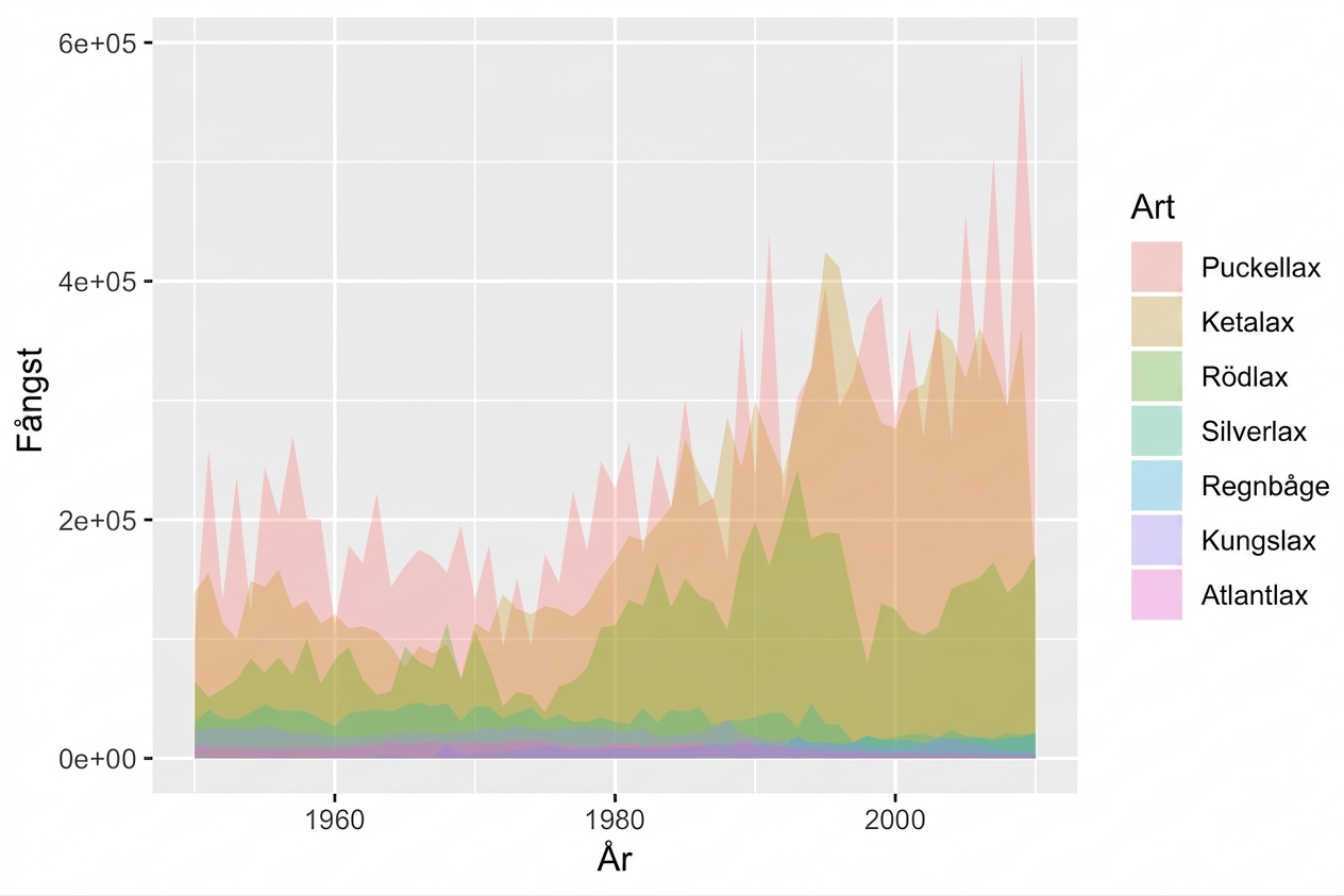
geom_ribbon()

ggplot(fish, aes(x = Year, 
                 y = Capture, 
                 fill = Species)) + 
  geom_ribbon(aes(ymax = Capture, 
                  ymin = 0), 
              alpha = 0.3)

Nu kör vi en övning!

Introduktion till datavisualisering med ggplot2