आपको logistic regression क्यों चाहिए

R में Regression परिचय

Richie Cotton

Data Evangelist at DataCamp

बैंक churn डेटासेट

has_churned	time_since_first_purchase	time_since_last_purchase
0	0.3993247	-0.5158691
1	-0.4297957	0.6780654
0	3.7383122	0.4082544
0	0.6032289	-0.6990435
...	...	...
response	संबंध की अवधि	गतिविधि की नवीनता

¹ https://www.rdocumentation.org/packages/bayesQR/topics/Churn

Churn बनाम recency: एक linear मॉडल

mdl_churn_vs_recency_lm <- lm(has_churned ~ time_since_last_purchase, data = churn)

Call:
lm(formula = has_churned ~ time_since_last_purchase, data = churn)

Coefficients:
             (Intercept)  time_since_last_purchase  
                 0.49078                   0.06378

coeffs <- coefficients(mdl_churn_vs_recency_lm)
intercept <- coeffs[1]
slope <- coeffs[2]

Linear मॉडल का विज़ुअलाइज़ेशन

ggplot(
  churn, 
  aes(time_since_last_purchase, has_churned)
) +
  geom_point() +
  geom_abline(intercept = intercept, slope = slope)

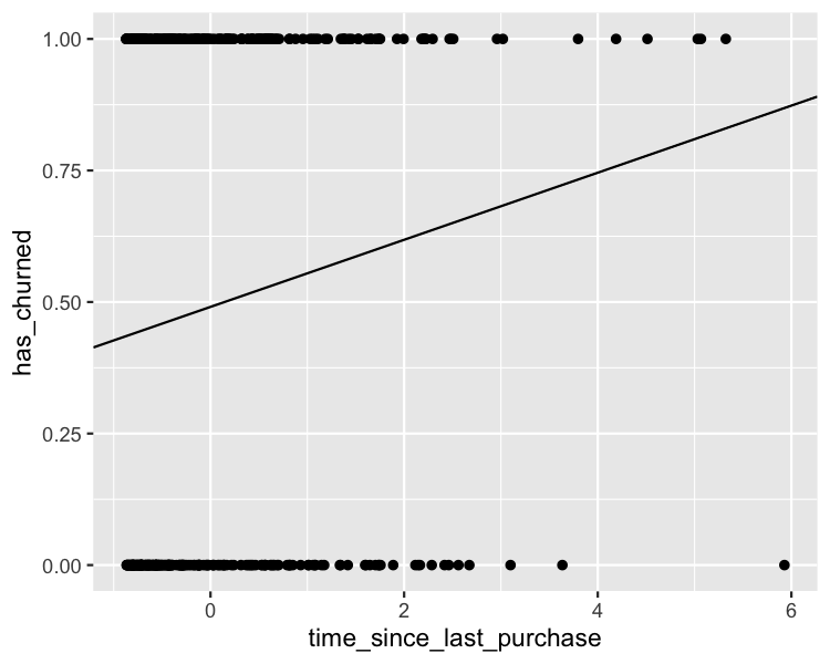
Predictions churn की probability हैं, churn की मात्रा नहीं.

ग्राहक ने churn किया या नहीं बनाम पिछली खरीद के बाद का समय का स्कैटर प्लॉट. सभी बिंदु y = 0 या y = 1 पर हैं. एक linear ट्रेंड लाइन दिखाती है कि पिछली खरीद से समय बढ़ने पर churn की probability बढ़ती है.

ज़ूम आउट करना

ggplot(
  churn, 
  aes(days_since_last_purchase, has_churned)
) +
  geom_point() +
  geom_abline(intercept = intercept, slope = slope) +
  xlim(-10, 10) +
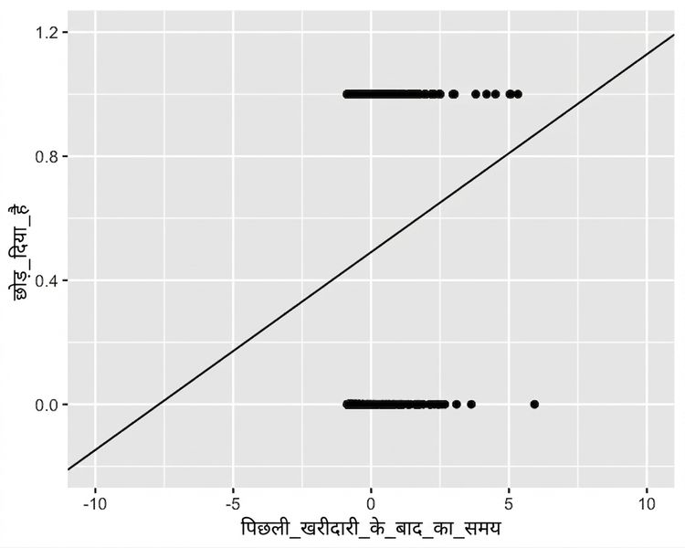
  ylim(-0.2, 1.2)

ग्राहक ने churn किया या नहीं बनाम पिछली खरीद के बाद का समय का वही स्कैटर प्लॉट. इस बार अक्ष ज़्यादा बाहर तक ज़ूम हैं, दिख रहा है कि ट्रेंड लाइन y = 0 से नीचे और y = 1 से ऊपर चली जाती है, जो असंभव होना चाहिए.

Logistic regression क्या है?

generalized linear model का एक और प्रकार.
जब response वैरिएबल logical हो.
responses logistic (S-आकार) कर्व का पालन करते हैं.

glm() के साथ linear regression

glm(has_churned ~ time_since_last_purchase, data = churn, family = gaussian)

Call:  glm(formula = has_churned ~ time_since_last_purchase, family = gaussian, 
    data = churn)

Coefficients:
             (Intercept)  time_since_last_purchase  
                 0.49078                   0.06378  

Degrees of Freedom: 399 Total (i.e. Null);  398 Residual
Null Deviance:        100 
Residual Deviance: 98.02     AIC: 578.7

Logistic regression: glm() में binomial family

mdl_recency_glm <- glm(has_churned ~ time_since_last_purchase, data = churn, family = binomial)

Call:  glm(formula = has_churned ~ time_since_last_purchase, family = binomial, 
    data = churn)

Coefficients:
             (Intercept)  time_since_last_purchase  
                -0.03502                   0.26921  

Degrees of Freedom: 399 Total (i.e. Null);  398 Residual
Null Deviance:        554.5 
Residual Deviance: 546.4     AIC: 550.4

Logistic मॉडल का विज़ुअलाइज़ेशन

ggplot(
  churn, 
  aes(time_since_last_purchase, has_churned)
) +
  geom_point() +
  geom_abline(
    intercept = intercept, slope = slope
  ) +
  geom_smooth(
    method = "glm", 
    se = FALSE, 
    method.args = list(family = binomial)
  )

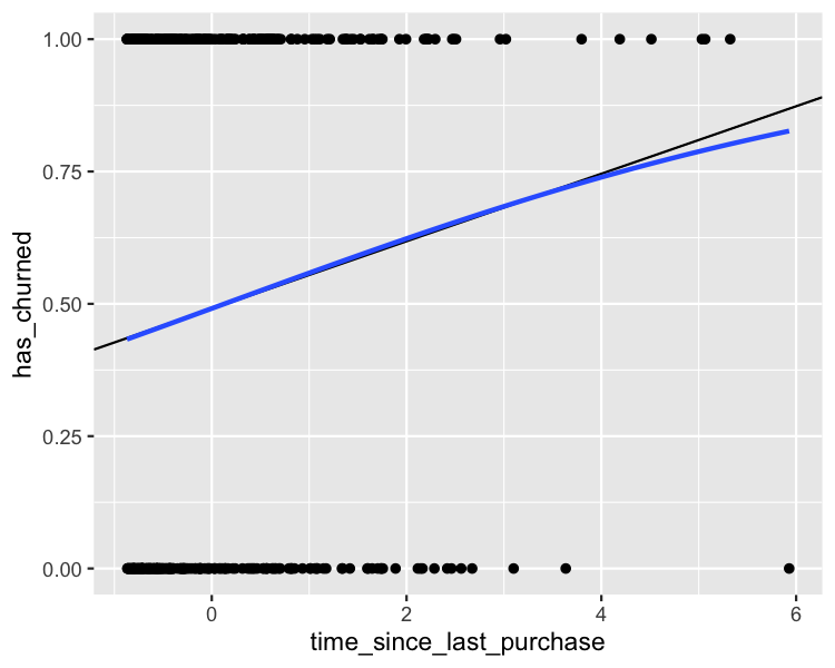
ग्राहक ने churn किया या नहीं बनाम पिछली खरीद के बाद का समय का स्कैटर प्लॉट. Linear और logistic दोनों ट्रेंड लाइनें दिखती हैं, और दोनों में समय बढ़ने पर churn की probability बढ़ती है. उच्च समय पर दोनों लाइनों में थोड़ा अंतर दिखता है.

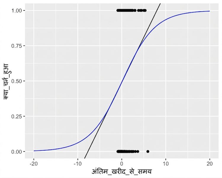
ज़ूम आउट करना

ग्राहक ने churn किया या नहीं बनाम पिछली खरीद के बाद का समय का स्कैटर प्लॉट, दोनों ट्रेंड लाइनों के साथ. अक्ष पहले से अधिक ज़ूम-आउट हैं, दिखता है कि logistic ट्रेंड लाइन कभी 0 से 1 की churn रेंज से बाहर नहीं जाती.

अभ्यास करते हैं!

R में Regression परिचय