आपको logistic regression क्यों चाहिए

Python में statsmodels के साथ Regression परिचय

Maarten Van den Broeck

Content Developer at DataCamp

Bank churn डेटासेट

has_churned	time_since_first_purchase	time_since_last_purchase
0	0.3993247	-0.5158691
1	-0.4297957	0.6780654
0	3.7383122	0.4082544
0	0.6032289	-0.6990435
...	...	...
response	length of relationship	recency of activity

¹ https://www.rdocumentation.org/packages/bayesQR/topics/Churn

Churn बनाम recency: एक linear मॉडल

mdl_churn_vs_recency_lm = ols("has_churned ~ time_since_last_purchase",
                              data=churn).fit()

print(mdl_churn_vs_recency_lm.params)

Intercept                   0.490780
time_since_last_purchase    0.063783
dtype: float64

intercept, slope = mdl_churn_vs_recency_lm.params

Linear मॉडल का विज़ुअलाइज़ेशन

sns.scatterplot(x="time_since_last_purchase",
                y="has_churned",
                data=churn)


plt.axline(xy1=(0, intercept),
           slope=slope)

plt.show()

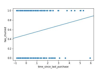
आखिरी खरीद के समय से लेकर churn तक का scatter plot. सभी पॉइंट y = 0 या y = 1 की रेखा पर हैं. एक linear ट्रेंड लाइन दिखाती है कि जैसे-जैसे आखिरी खरीद का समय बढ़ता है, churn की प्रायिकता बढ़ती है.

Zoom out करना

sns.scatterplot(x="time_since_last_purchase",
                y="has_churned",
                data=churn)

plt.axline(xy1=(0,intercept),
           slope=slope)


plt.xlim(-10, 10)
plt.ylim(-0.2, 1.2)

plt.show()

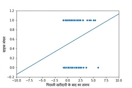
वही scatter plot, इस बार axes ज्यादा ज़ूम-आउट हैं. ट्रेंड लाइन y = 0 से नीचे और y = 1 से ऊपर जाती दिखती है, जो असंभव होना चाहिए.

Logistic regression क्या है?

generalized linear model का एक और प्रकार.
जब response वैरिएबल logical हो.
responses logistic (S-आकार) कर्व का पालन करते हैं.

logit() से logistic regression

from statsmodels.formula.api import logit
mdl_churn_vs_recency_logit = logit("has_churned ~ time_since_last_purchase",
                                   data=churn).fit()

print(mdl_churn_vs_recency_logit.params)

Intercept                  -0.035019
time_since_last_purchase    0.269215
dtype: float64

Logistic मॉडल का विज़ुअलाइज़ेशन

sns.regplot(x="time_since_last_purchase",
            y="has_churned",
            data=churn,
            ci=None,
            logistic=True)

plt.axline(xy1=(0,intercept),
           slope=slope,
           color="black")

plt.show()

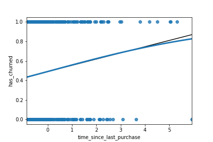
churn बनाम आखिरी खरीद का समय वाला scatter plot. Linear और logistic दोनों ट्रेंड लाइनें दिखती हैं, और दोनों में समय बढ़ने पर churn की प्रायिकता बढ़ती है. अधिक समय के मानों पर छोड़कर, दोनों रेखाएँ काफी मिलती-जुलती हैं.

Zoom out करना

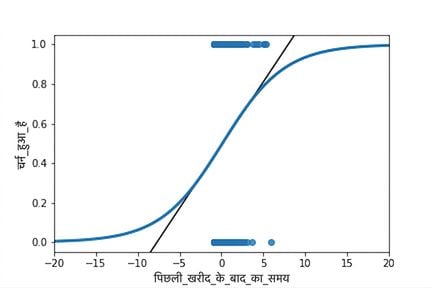
वही scatter plot, दोनों ट्रेंड लाइनों के साथ. axes अब ज़्यादा ज़ूम-आउट हैं और logistic ट्रेंड लाइन कभी भी 0 से 1 की churn रेंज के बाहर नहीं जाती.

अभ्यास करते हैं!

Python में statsmodels के साथ Regression परिचय