Кількісна оцінка якості логістичної регресії

Вступ до Regression у R

Richie Cotton

Data Evangelist at DataCamp

Чотири результати

	actual false	actual true
predicted false	correct	false negative
predicted true	false positive	correct

Матриця помилок: підрахунок результатів

mdl_recency <- glm(has_churned ~ time_since_last_purchase, data = churn, family = "binomial")

actual_response <- churn$has_churned

predicted_response <- round(fitted(mdl_recency))

outcomes <- table(predicted_response, actual_response)

                  actual_response
predicted_response   0   1
                 0 141 111
                 1  59  89

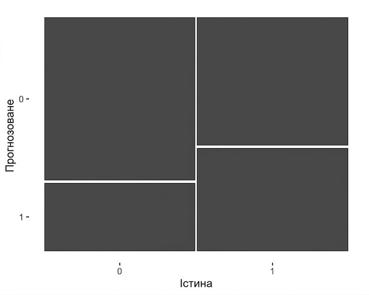
Візуалізація матриці помилок: мозаїчний графік

library(ggplot2)
library(yardstick)

confusion <- conf_mat(outcomes)

                  actual_response
predicted_response   0   1
                 0 141 111
                 1  59  89

autoplot(confusion)

Мозаїчний графік результатів моделі churn проти recency. Є по 200 спостережень для справжніх відтоків і справжніх не-відтоків, тож кожен стовпчик має однакову ширину.

Показники якості

summary(confusion, event_level = "second")

# A tibble: 13 x 3
   .metric              .estimator .estimate
   <chr>                <chr>          <dbl>
 1 accuracy             binary         0.575
 2 kap                  binary         0.150
 3 sens                 binary         0.445
 4 spec                 binary         0.705
 5 ppv                  binary         0.601
 6 npv                  binary         0.560
 7 mcc                  binary         0.155
 8 j_index              binary         0.150
 9 bal_accuracy         binary         0.575
10 detection_prevalence binary         0.37 
11 precision            binary         0.601
12 recall               binary         0.445
13 f_meas               binary         0.511

Точність (Accuracy)

summary(confusion) %>% 
  slice(1)

# A tibble: 3 x 3
  .metric  .estimator .estimate
  <chr>    <chr>          <dbl>
1 accuracy binary         0.575

Accuracy — частка правильних передбачень.

$$ accuracy = \frac{TN + TP}{TN + FN + FP + TP} $$

confusion

                  actual_response
predicted_response   0   1
                 0 141 111
                 1  59  89

(141 + 89) / (141 + 111 + 59 + 89)

0.575

Чутливість (Sensitivity)

summary(confusion) %>% 
  slice(3)

# A tibble: 1 x 3
  .metric .estimator .estimate
  <chr>   <chr>          <dbl>
1 sens    binary         0.445

Sensitivity — частка справжніх спрацьовувань (true positives).

$$ sensitivity = \frac{TP}{FN + TP} $$

confusion

                  actual_response
predicted_response   0   1
                 0 141 111
                 1  59  89

89 / (111 + 89)

0.445

Специфічність (Specificity)

summary(confusion) %>% 
  slice(4)

# A tibble: 1 x 3
  .metric .estimator .estimate
  <chr>   <chr>          <dbl>
1 spec    binary         0.705

Specificity — частка справжніх негативів.

$$ specificity = \frac{TN}{TN + FP} $$

confusion

                  actual_response
predicted_response   0   1
                 0 141 111
                 1  59  89

141 / (141 + 59)

0.705

Давайте потренуємось!

Вступ до Regression у R