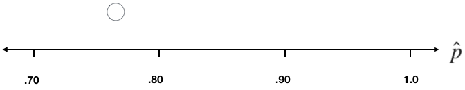
Interpreting a Confidence Interval
Inference for Categorical Data in R

Andrew Bray
Assistant Professor of Statistics at Reed College
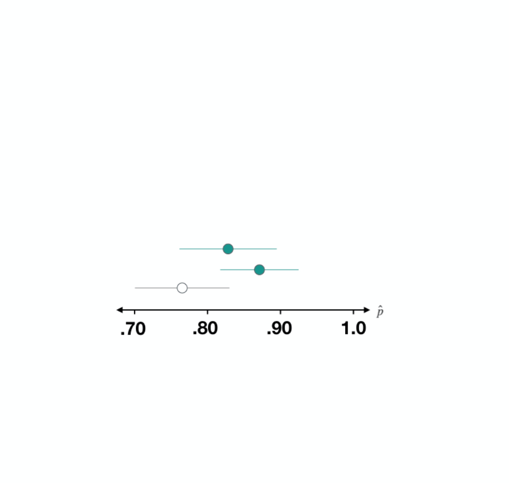
Dataset 1


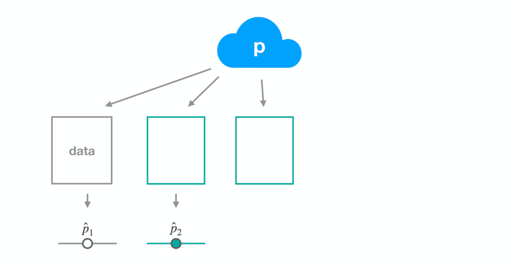
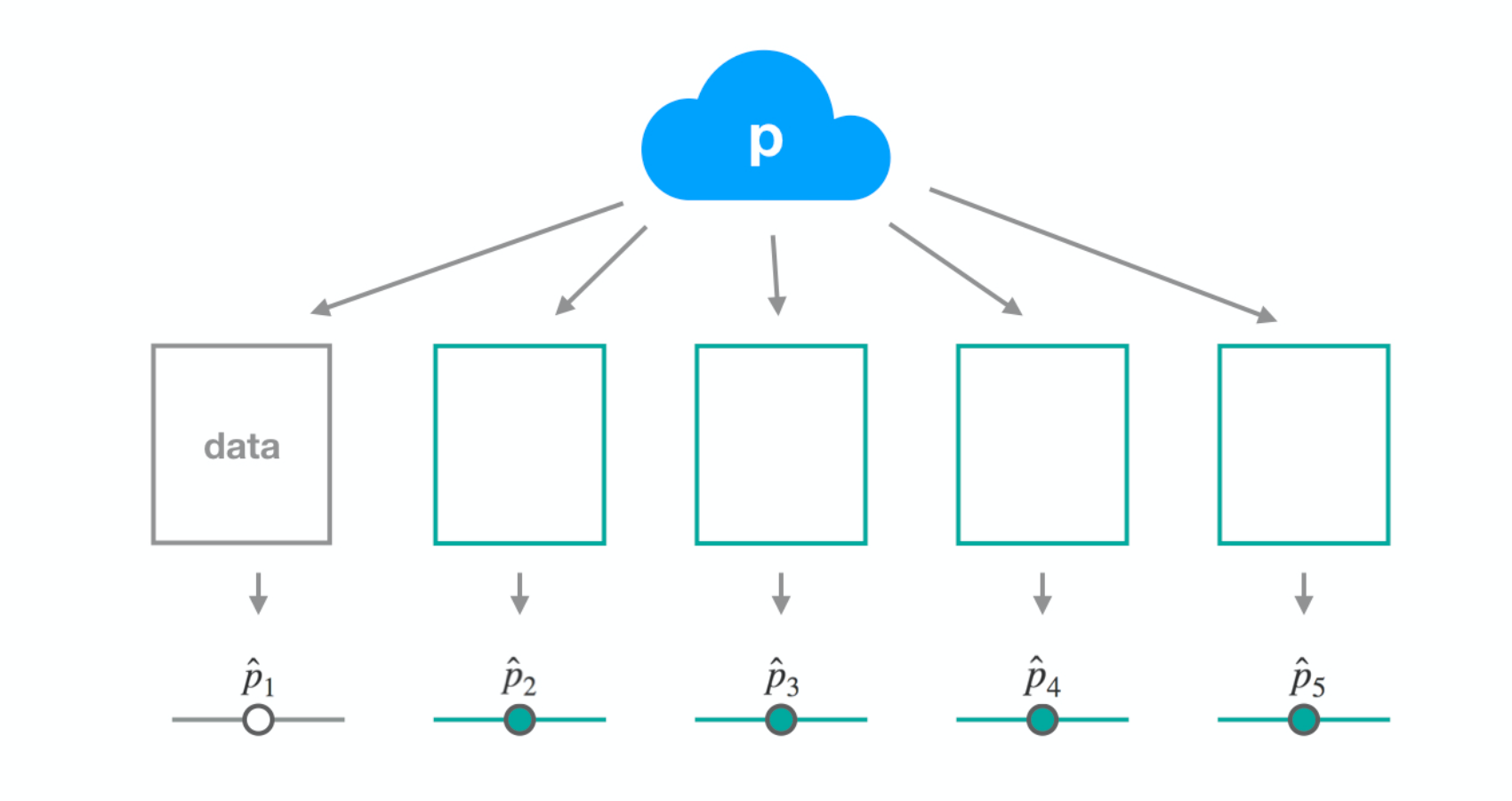
Dataset 2
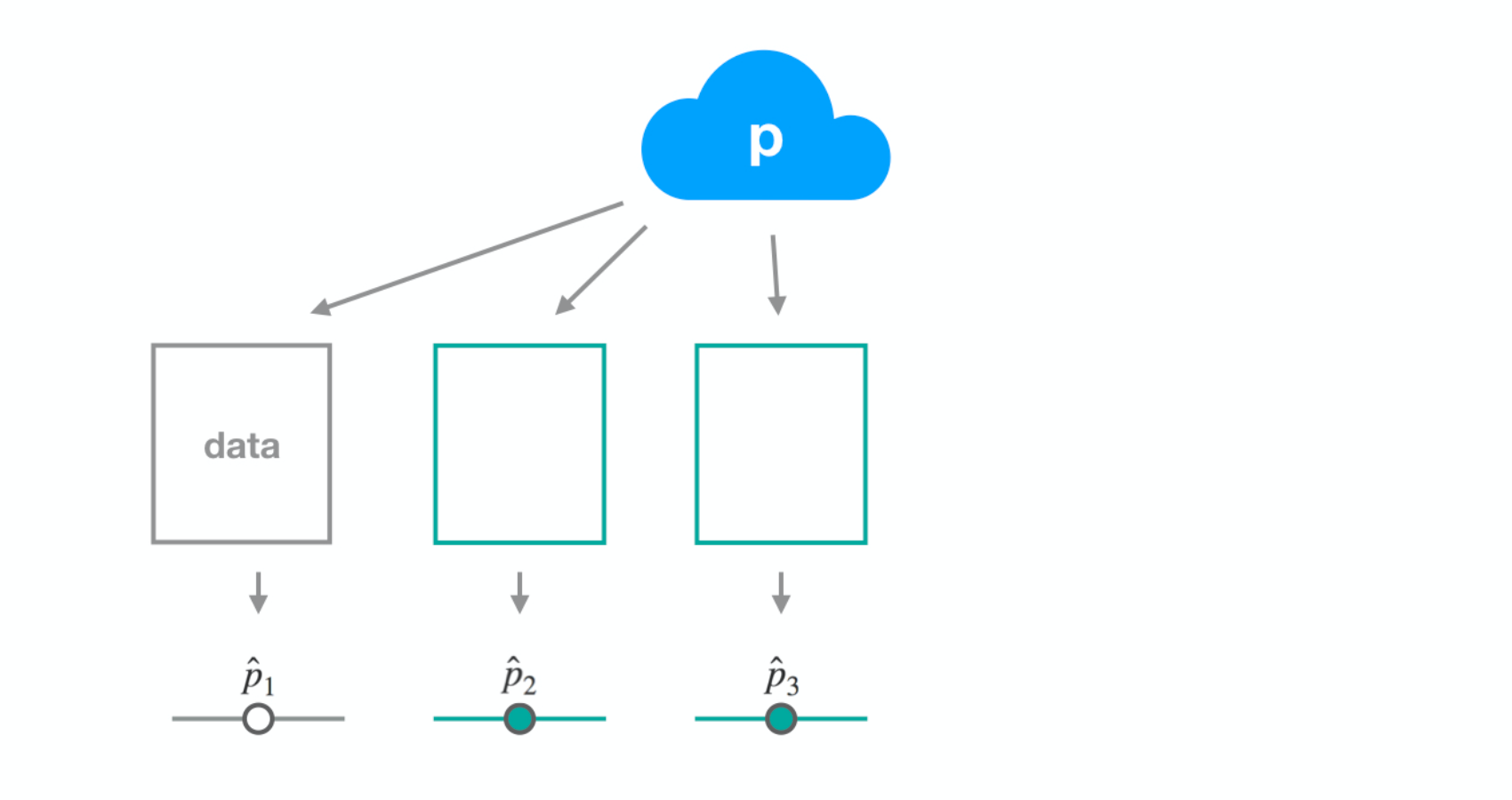
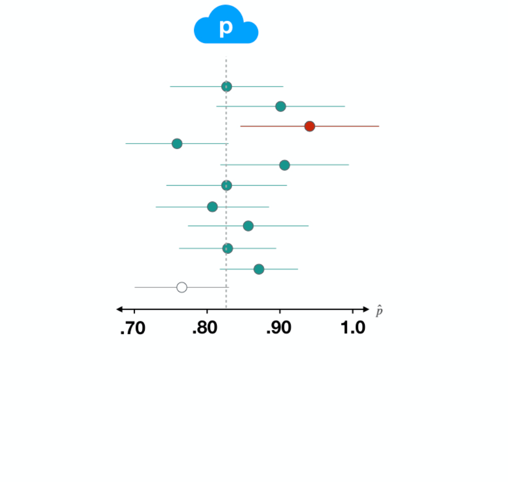
Dataset 3
Dataset 3
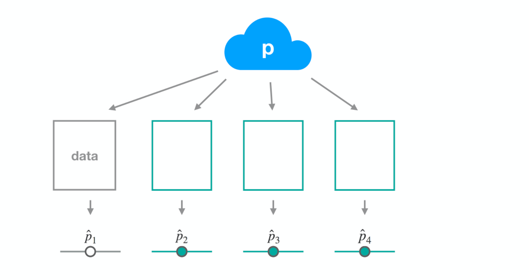
Dataset 3
Dataset 3
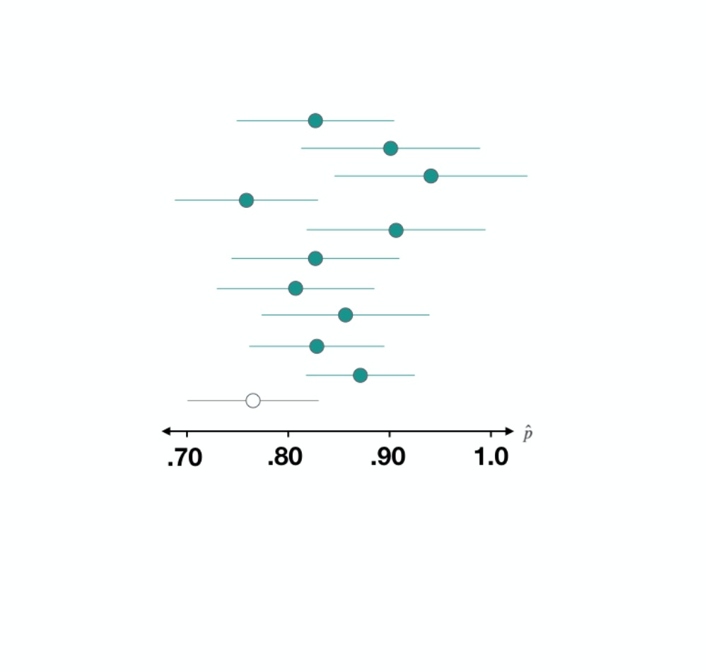
Dataset 3
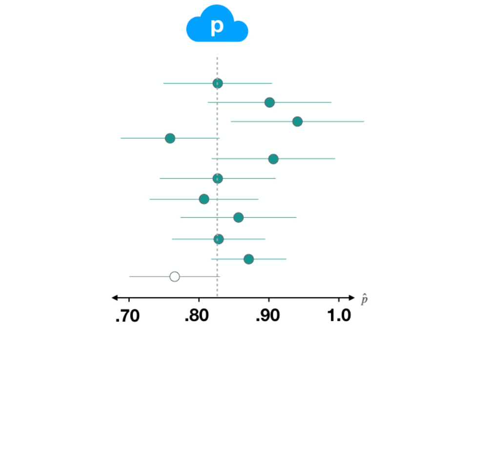
Dataset 3
Inference for Categorical Data in R
Andrew Bray
Assistant Professor of Statistics at Reed College

