The General Social Survey
Inference for Categorical Data in R

Andrew Bray
Assistant Professor of Statistics at Reed College


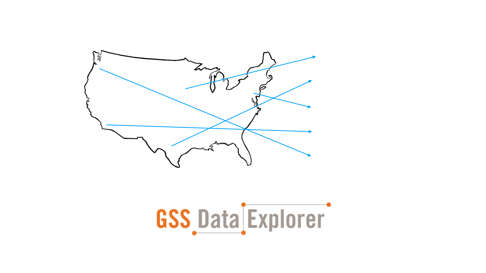
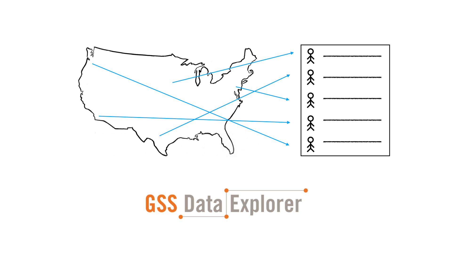
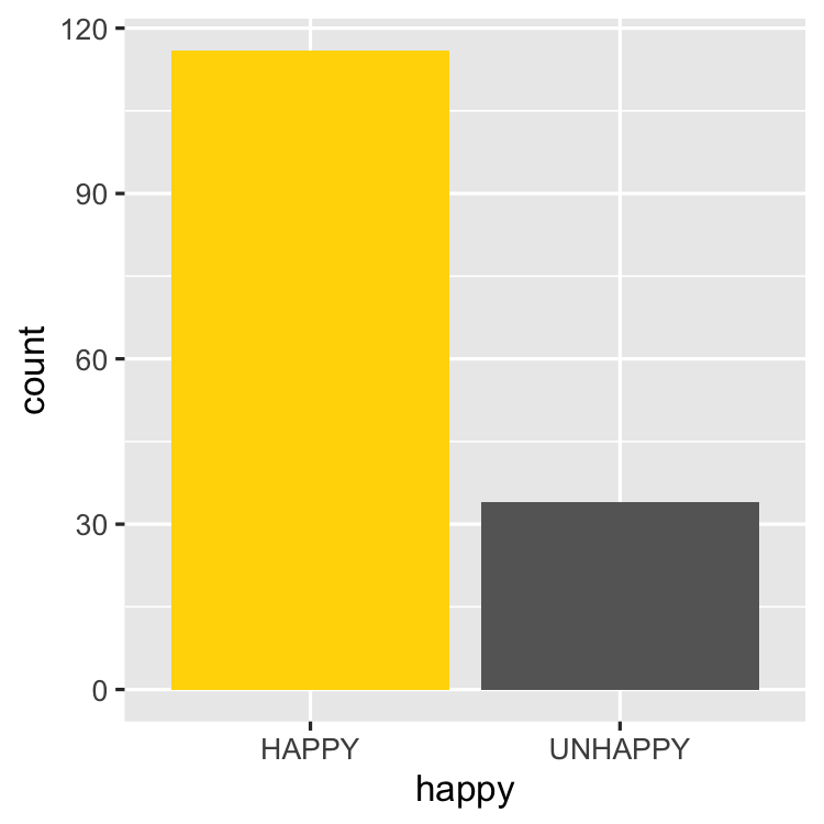
Exploring GSS
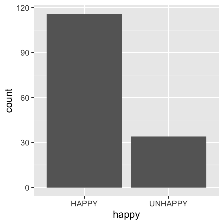
Exploring GSS
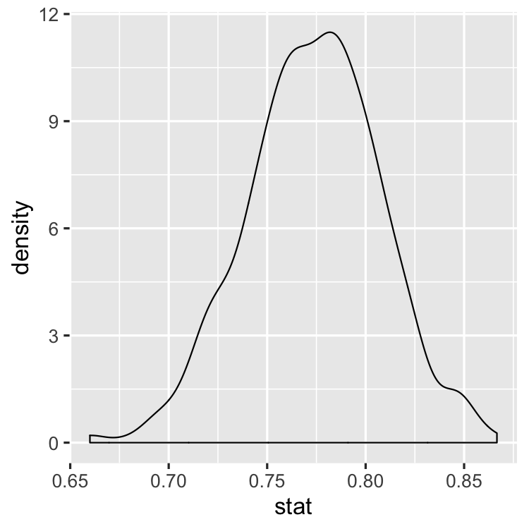
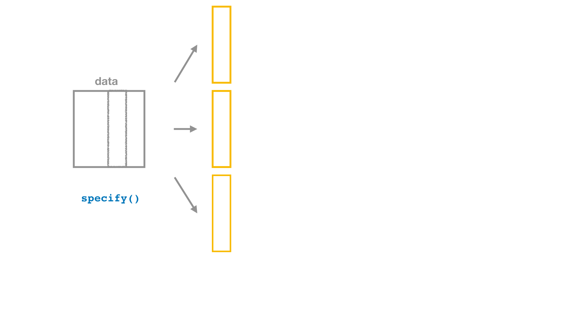
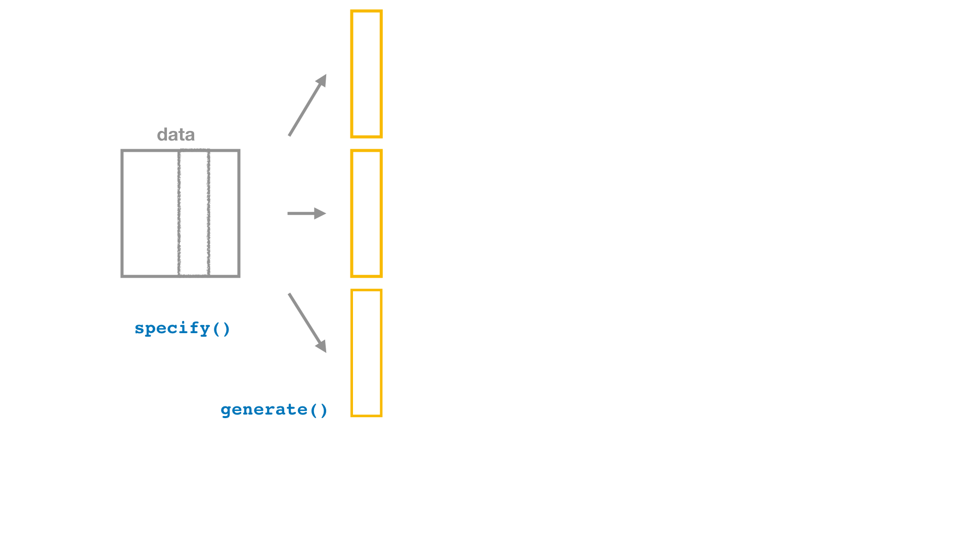
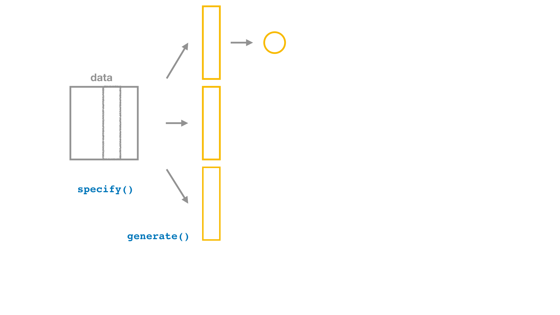
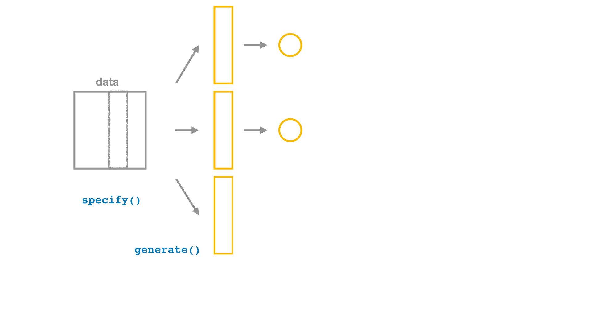
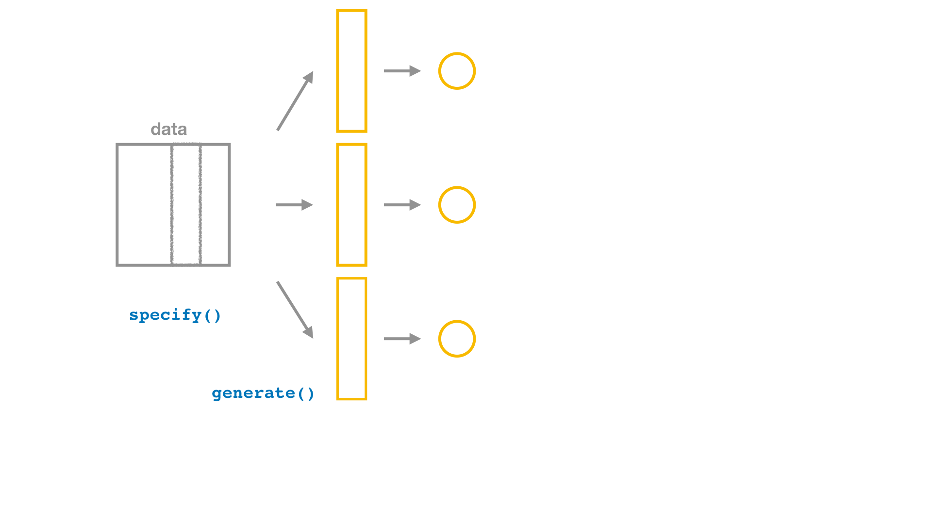
Bootstrap

Bootstrap
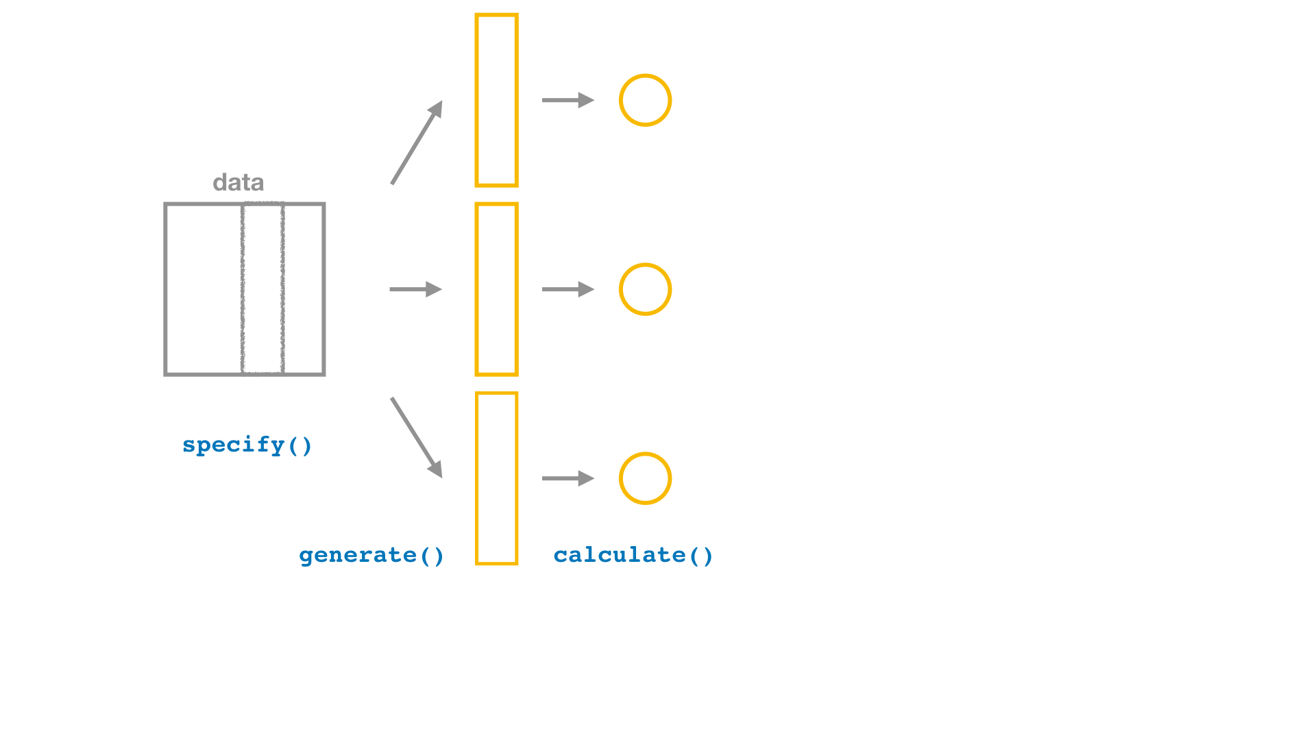
Bootstrap
Bootstrap
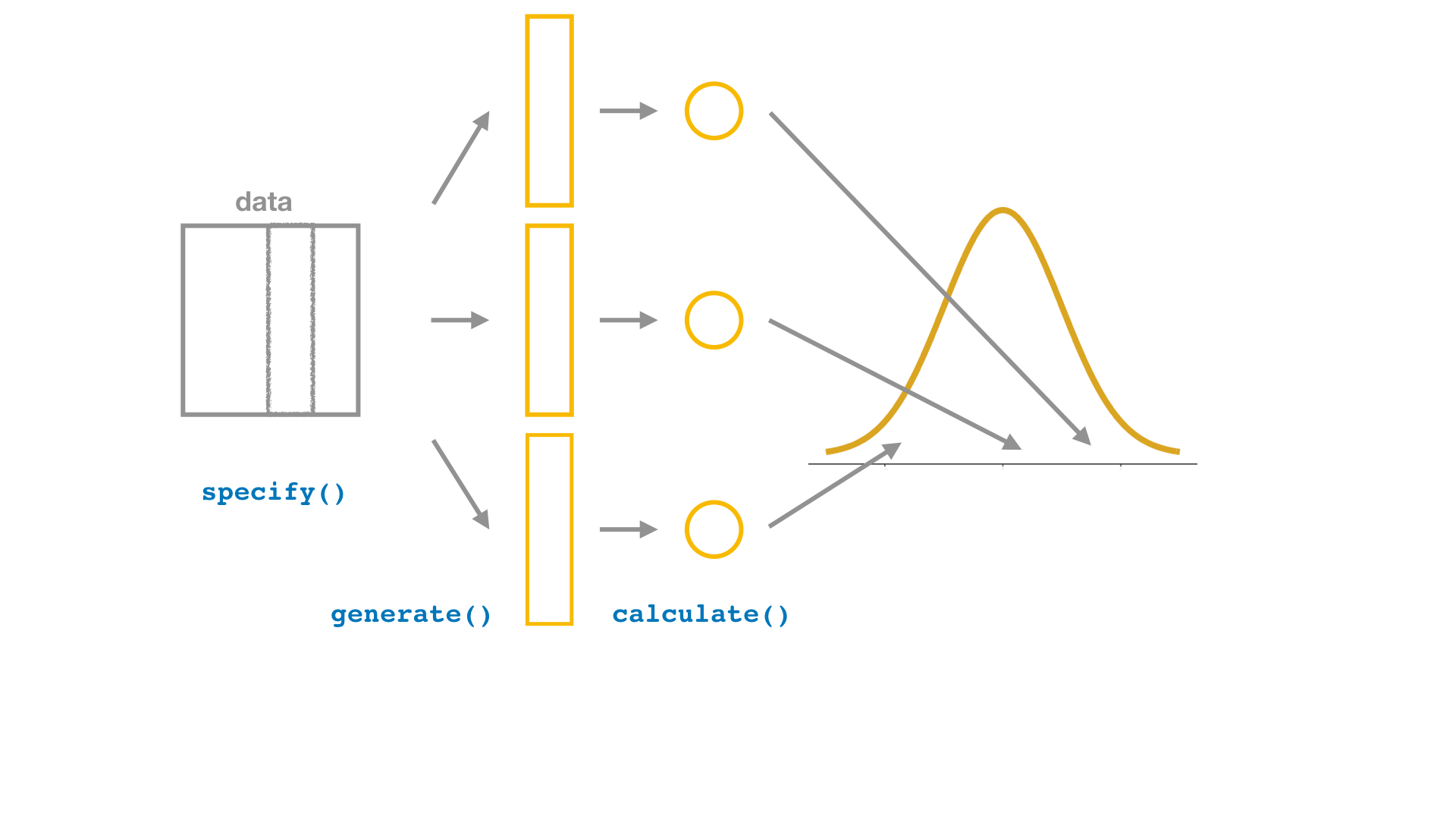
Bootstrap
Bootstrap
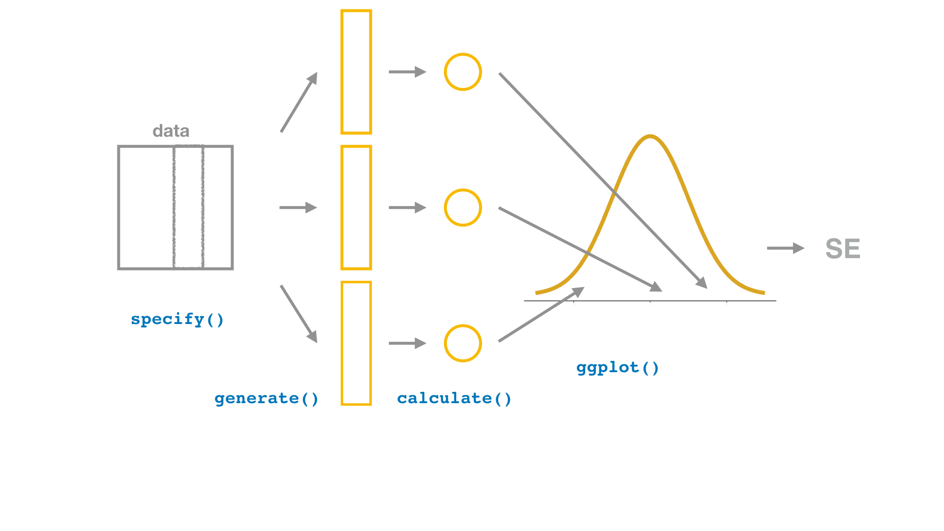
Bootstrap
Bootstrap
Bootstrap
Bootstrap
Bootstrap
Bootstrap

Bootstrap
Bootstrap
Bootstrap Confidence Interval