R 中的时间序列数据处理
Harrison Brown
Graduate Researcher in Geography
频率:
时间分辨率:
mean
sum
max
xts:
xts
zoo
apply.*()
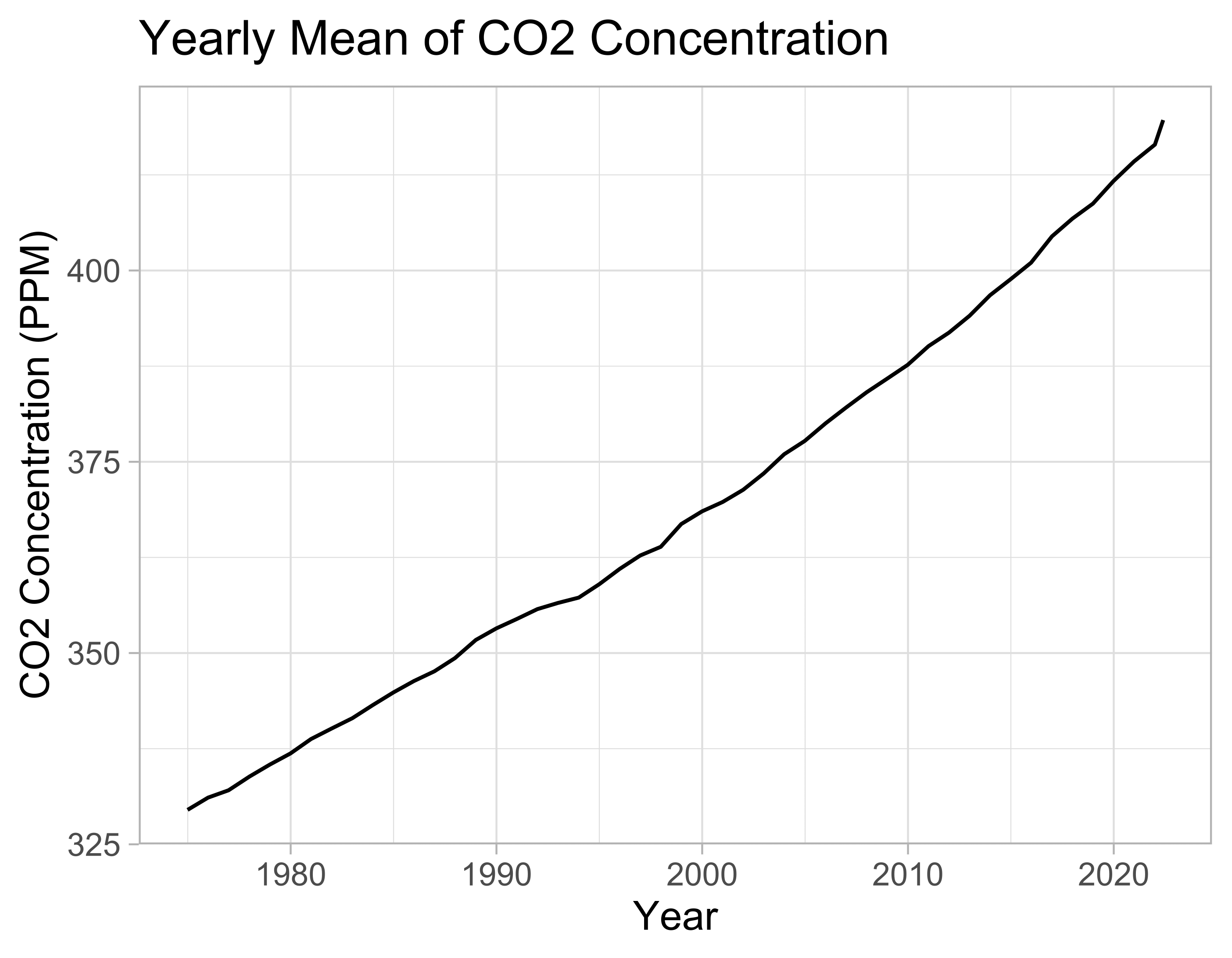
yearly_mean <-
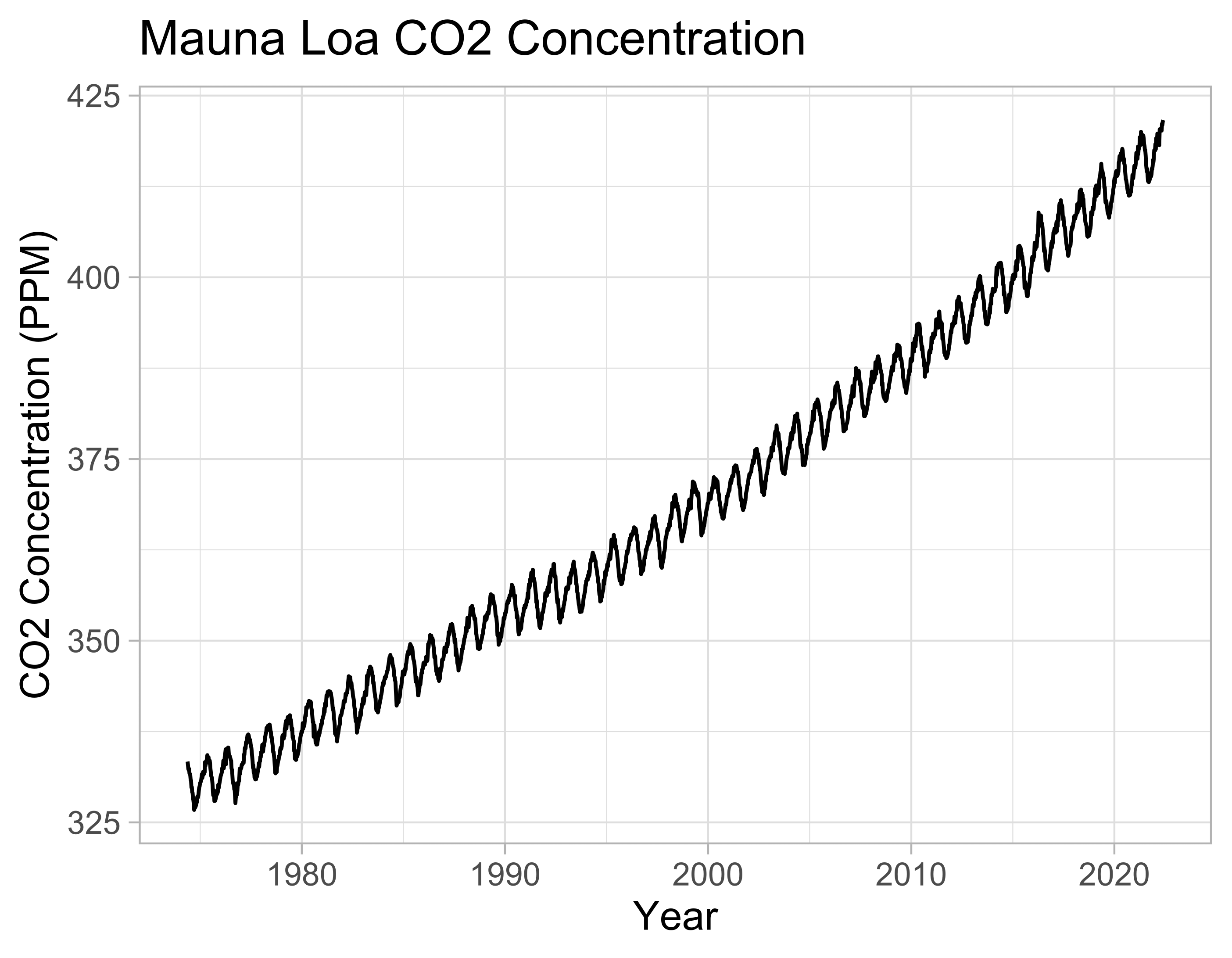
  apply.yearly(x = maunaloa,
               FUN = mean)
autoplot(yearly_mean) +
  labs(...)
daily_total <-
  apply.daily(hourly_sales,
              FUN = sum)
weekly_max <-
  apply.weekly(daily_temperature,
               FUN = max)
monthly_average <-
  apply.monthly(daily_price,
               FUN = mean)
apply.quarterly(sales_report,
                FUN = sum)
apply.yearly(monthly_salary,
             FUN = sum)
xts::endpoints()
xts::period.apply()
biweekly_eps <-
  endpoints(x = daily_data,
            on = "weeks",
            k = 2)
biweekly_data <-
  period.apply(x = daily_data,
               INDEX = biweekly_eps,
               FUN = mean)
biweekly_data
2002-05-05 8.148611
2002-05-19 8.146776
2002-06-02 8.060020
2002-06-16 8.028224
2002-06-30 7.944792
2002-07-14 7.930159
...