季节性 ARIMA 模型

R 中的预测

Rob J. Hyndman

Professor of Statistics at Monash University

ARIMA 模型

ch4_vid3_slides.003.png

d = 一阶差分数
p = 普通 AR 滞后数：
q = 普通 MA 滞后数：

ARIMA 模型

ch4_vid3_slides.007.png

d = 一阶差分数
p = 普通 AR 滞后数：
q = 普通 MA 滞后数：

ARIMA 模型

ch4_vid3_slides.008.png

d = 一阶差分数
p = 普通 AR 滞后数：$\ y_{t-1}, y_{t-2},...,y_{t-p}$
q = 普通 MA 滞后数：$\ \epsilon_{t-1}, \epsilon_{t-2},...,\epsilon_{t-q}$
D = 季节差分数
P = 季节 AR 滞后数：$\ y_{t-m}, y_{t-2m},...,y_{t-Pm}$
Q = 季节 MA 滞后数：$\ \epsilon_{t-m}, \epsilon_{t-2m},...,\epsilon_{t-Qm}$
m = 年内观测数

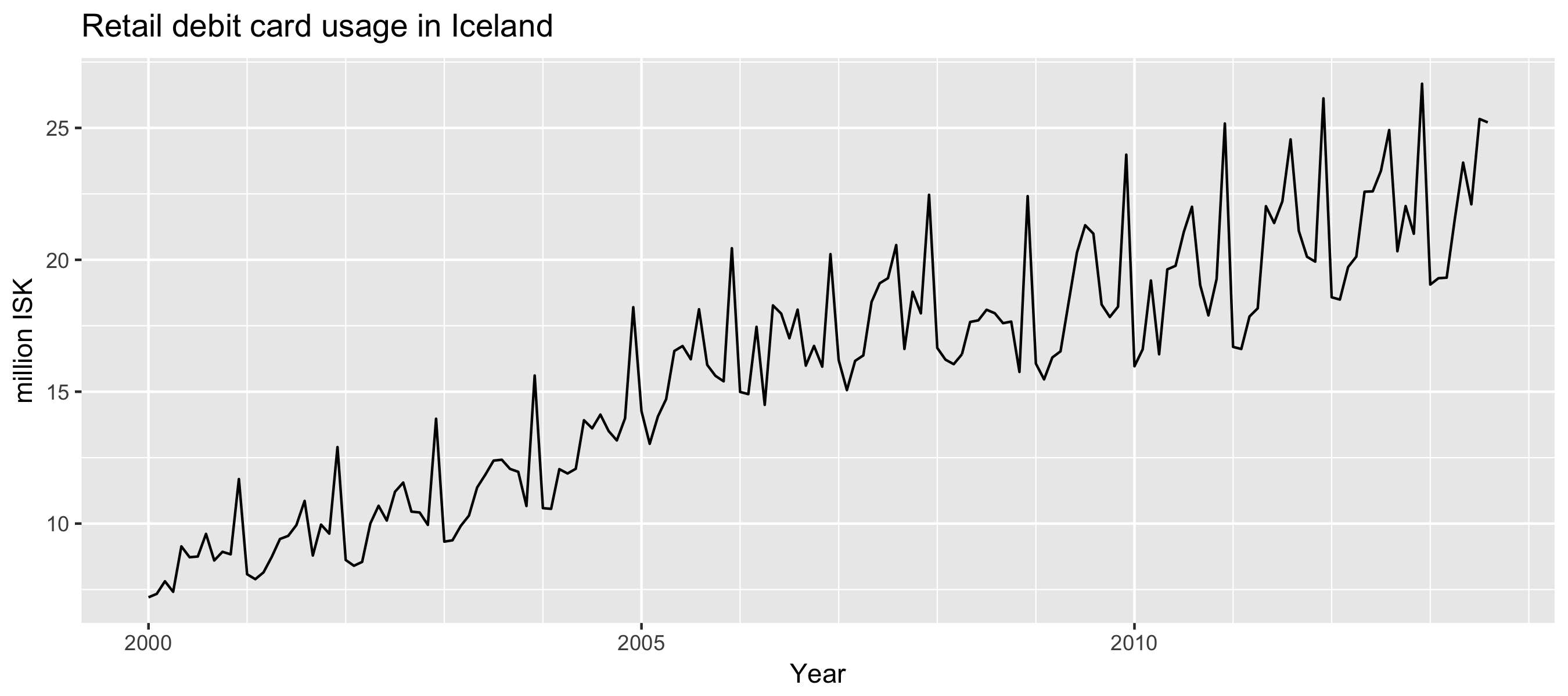
例子：冰岛每月零售借记卡使用量

autoplot(debitcards) +
  xlab("Year") + ylab("million ISK") +
  ggtitle("Retail debit card usage in Iceland")

例子：冰岛每月零售借记卡使用量

fit <- auto.arima(debitcards, lambda = 0)
fit

Series: debitcards
ARIMA(0,1,4)(0,1,1)[12]
Box Cox transformation: lambda= 0
Coefficients:
         ma1    ma2    ma3     ma4    sma1
      -0.796  0.086  0.263  -0.175  -0.814
s.e.   0.082  0.099  0.100   0.080   0.112
sigma^2 estimated as 0.00232:  log likelihood=239.3
AIC=-466.7   AICc=-466.1   BIC=-448.6

例子：冰岛每月零售借记卡使用量

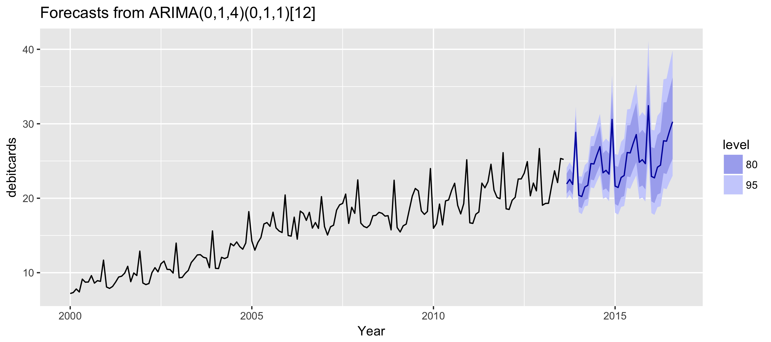
fit %>%
  forecast(h = 36) %>%
  autoplot() + xlab("Year")

Vamos praticar!

R 中的预测