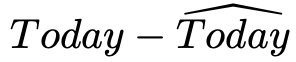
MA 模型的估计与预测

R 中的时间序列分析

David S. Matteson

Associate Professor at Cornell University

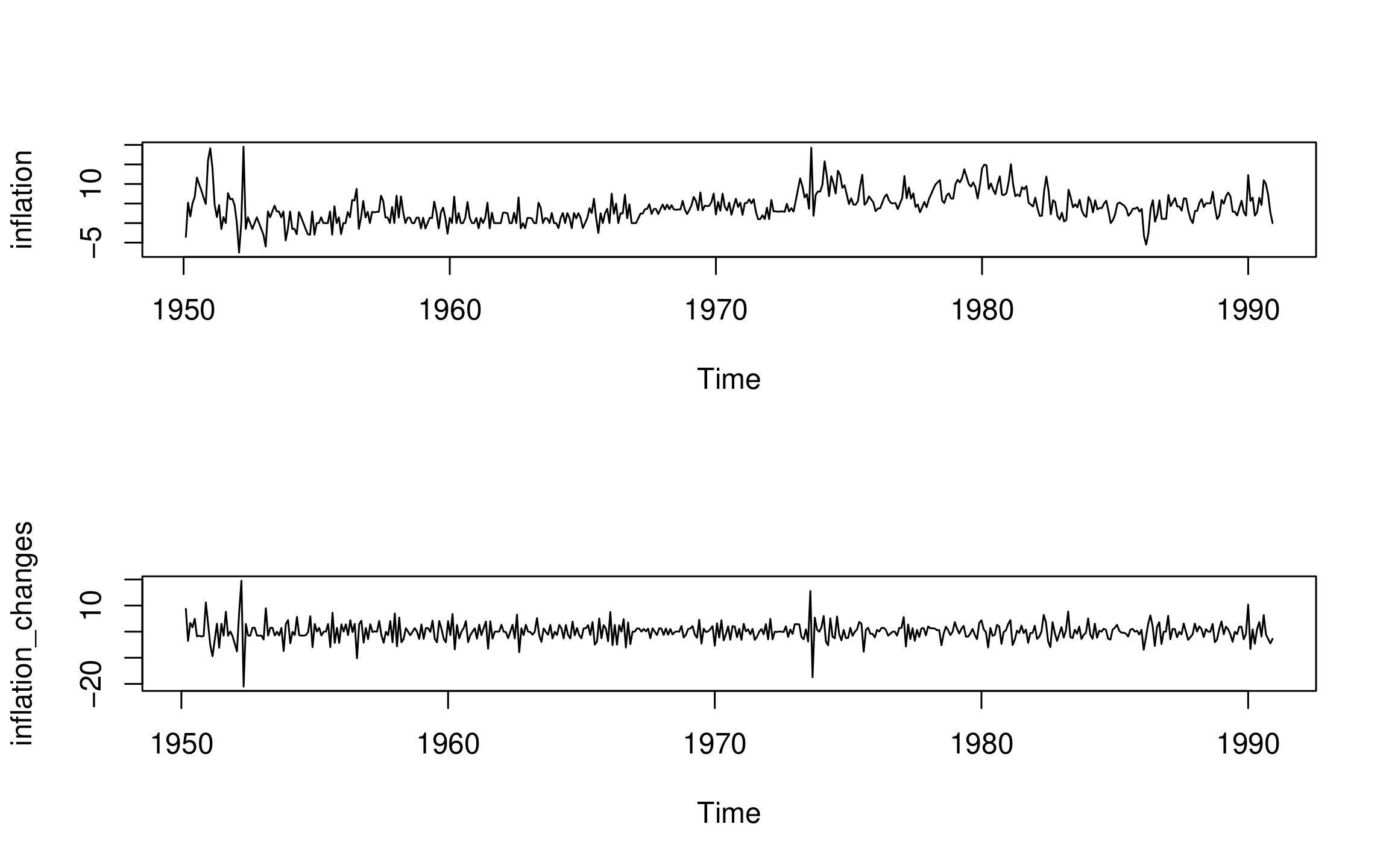
美国月度通胀率（百分比，年化）
月度观测：1950–1990 年

data(Mishkin, package = "Ecdat")
inflation <- as.ts(Mishkin[, 1])

inflation_changes <- diff(inflation)

ts.plot(inflation) ; ts.plot(inflation_changes)

MA 过程：通胀率变动 - II

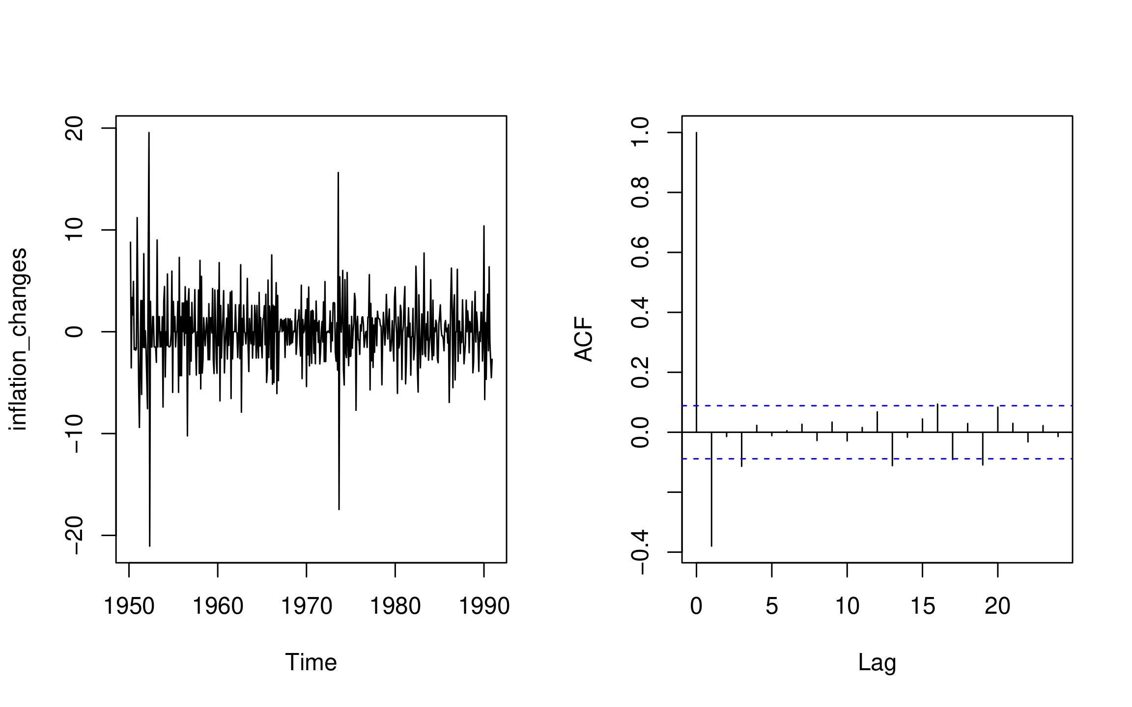
Inflation_changes：美国月度通胀率的变动
绘制序列及其样本 ACF：

ts.plot(inflation_changes)
acf(inflation_changes, lag.max = 24)

$今天 = 均值 + 噪声 + 斜率 ×（昨天的噪声）$ $$Y_t = \mu + \epsilon_t + \theta\epsilon_{t-1}$$ $$\epsilon_t ~ WhiteNoise(0, \sigma_{\epsilon}^2)$$

MA_inflation_changes <- arima(inflation_changes, 
                              order = c(0, 0, 1))

print(MA_inflation_changes)

Coefficients:
         ma1  intercept
      -0.7932    0.0010
s.e.   0.0355    0.0281
sigma^2 estimated as 8.882

ma1 = $\hat{\theta}$，intercept = $\hat{\mu}$，sigma^2 = $\hat{\sigma^2_{\epsilon}}$

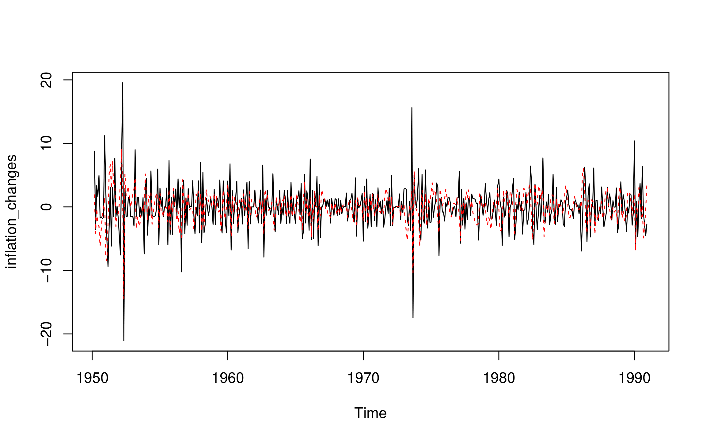
MA 过程：拟合值 - I

MA 拟合值：

$$\hat{Y_t} = \hat{\mu} +\hat{\theta}\hat{\epsilon_{t-1}}$$

残差 =

$$\hat{\epsilon_t} = Y_t - \hat{Y_t}$$

ts.plot(inflation_changes)
MA_inflation_changes_fitted <- 
    inflation_changes - residuals(MA_inflation_changes)

points(MA_inflation_changes_fitted, type = "l", 
       col = "red", lty = 2)

预测

向前 1 步预测：

predict(MA_inflation_changes)$pred

Jan
1991 4.831632

predict(MA_inflation_changes)$se

Jan
1991 2.980203

预测（续）

向前 h 步预测：

predict(MA_inflation_changes, n.ahead = 6)$pred

           Jan       Feb       Mar       Apr       May       Jun
1991  4.831632  0.001049  0.001049  0.001049  0.001049  0.001049

predict(MA_inflation_changes, n.ahead = 6)$se

           Jan       Feb       Mar       Apr       May       Jun
1991  2.980203  3.803826  3.803826  3.803826  3.803826  3.803826

让我们练习吧！

R 中的时间序列分析