AR 模型估计与预测

R 中的时间序列分析

David S. Matteson

Associate Professor at Cornell University

AR 过程:通胀率

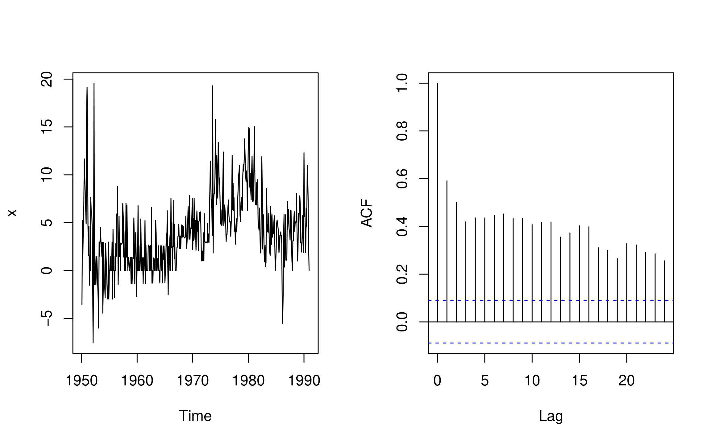
  • 美国月度通胀率(百分比,年化)。
  • 1950–1990 的月度观测
data(Mishkin, package = "Ecdat")

inflation <- as.ts(Mishkin[, 1])
ts.plot(inflation) ; acf(inflation)

R 中的时间序列分析

$$ (今日 - 均值) = 斜率 * (昨日 - 均值) + 噪声 $$

$$Y_t - \mu = \phi(Y_{t-1} - \mu) + \epsilon_t $$

$$\epsilon_t~ WhiteNoise(0, \sigma_{\epsilon}^2)$$

AR_inflation <- arima(inflation, order = c(1, 0, 0))

print(AR_inflation)
系数:
        ar1  intercept
     0.5960     3.9745
s.e. 0.0364        0.3471
sigma^2 估计为 9.713

ar1 = $ \hat{\phi}$,intercept = $ \hat{\mu} $,sigma^2 = $\hat{\sigma}^2_{\epsilon}$

R 中的时间序列分析

AR 过程:拟合值 - I

  • AR 拟合值:

$$\hat{Y_t} = \hat{\mu} + \hat{\phi}(Y_{t-1} - \hat{\mu})$$

  • 残差 =

$$ \hat{\epsilon_t} = Y_t - \hat{Y_t}$$

R 中的时间序列分析

AR 过程:拟合值 - II

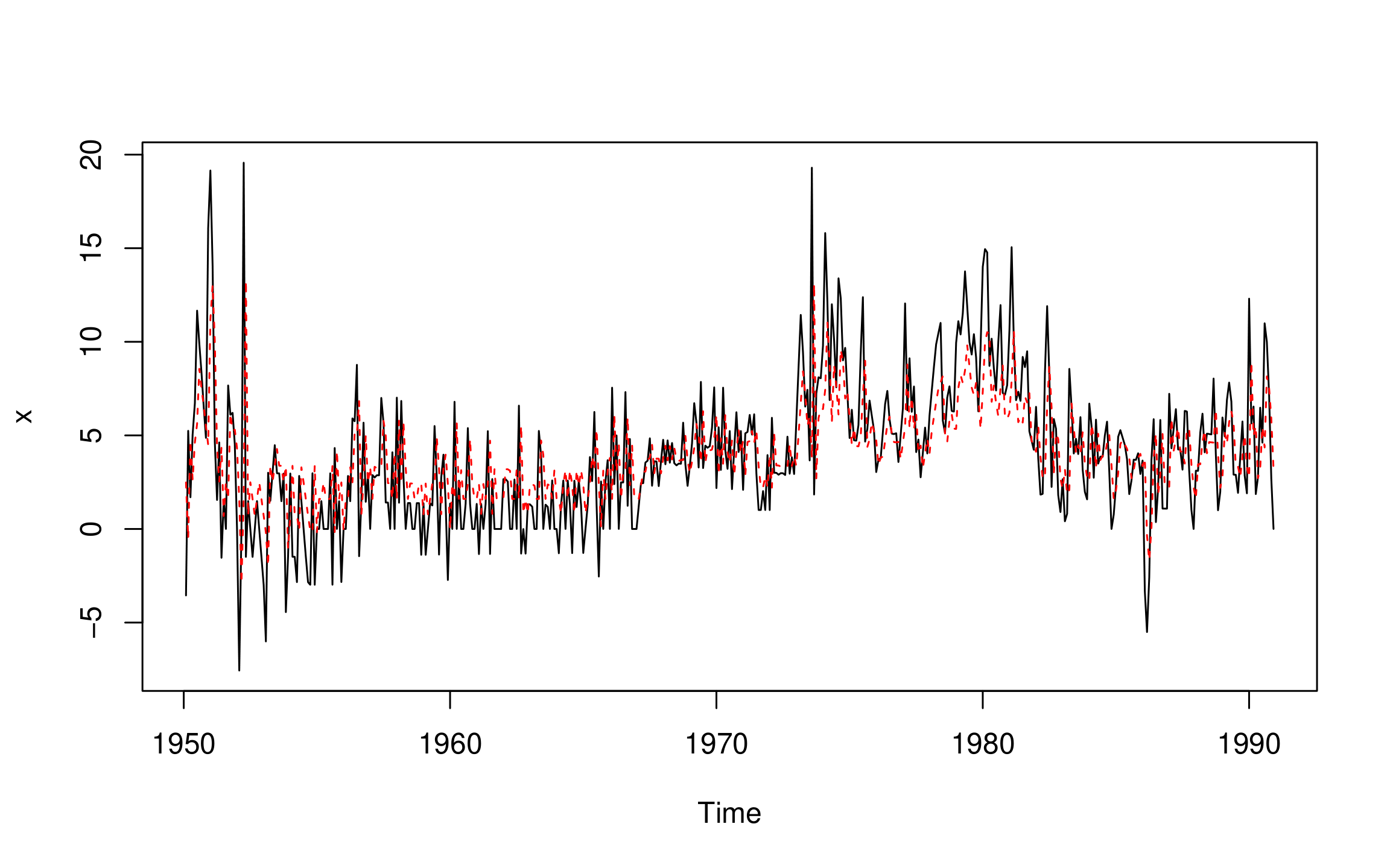
ts.plot(inflation)

AR_inflation_fitted <- inflation - residuals(AR_inflation)
points(AR_inflation_fitted, type = "l" col = "red", lty = 2)
R 中的时间序列分析

预测

  • 1 步超前预测
predict(AR_inflation)$pred 
Jan
1991 1.605797
predict(AR_inflation)$se
Jan
1991 3.116526
R 中的时间序列分析

预测(续)

  • h 步超前预测
predict(AR_inflation, n.ahead = 6)$pred
           Jan       Feb       Mar       Apr       May       Jun
1991  1.605797  2.562810  3.133165  3.473082  3.675664  3.796398
predict(AR_inflation, n.ahead = 6)$se
           Jan       Feb       Mar       Apr       May       Jun
1991  3.116526  3.628023  3.793136  3.850077  3.870101  3.877188

R 中的时间序列分析

Passons à la pratique !

R 中的时间序列分析

Preparing Video For Download...