两个数值型自变量

Python 中级回归：使用 statsmodels

Maarten Van den Broeck

Content Developer at DataCamp

可视化三个数值变量

3D 散点图
2D 散点图，用颜色表示响应

鱼数据集的另一列

species	mass_g	length_cm	height_cm
Bream	1000	33.5	18.96
Bream	925	36.2	18.75
Roach	290	24.0	8.88
Roach	390	29.5	9.48
Perch	1100	39.0	12.80
Perch	1000	40.2	12.60
Pike	1250	52.0	10.69
Pike	1650	59.0	10.81

3D 散点图

所有鱼类物种的 3D 散点图，轴为长度、质量和高度。该图在二维平面上难以解读。

二维散点图，颜色表示响应

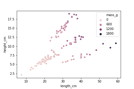
sns.scatterplot(x="length_cm", 
                y="height_cm",
                data=fish,
                hue="mass_g")

二维散点图，用颜色显示质量以可视化第三个数值变量。

包含两个数值型自变量的建模

mdl_mass_vs_both = ols("mass_g ~ length_cm + height_cm",
                       data=fish).fit()

print(mdl_mass_vs_both.params)

Intercept   -622.150234
length_cm     28.968405
height_cm     26.334804

预测流程

from itertools import product

length_cm = np.arange(5, 61, 5)
height_cm = np.arange(2, 21, 2)

p = product(length_cm, height_cm)

explanatory_data = pd.DataFrame(p,
                                columns=["length_cm",
                                         "height_cm"])

prediction_data = explanatory_data.assign(
  mass_g = mdl_mass_vs_both.predict(explanatory_data))

print(prediction_data)

     length_cm  height_cm       mass_g
0            5          2  -424.638603
1            5          4  -371.968995
2            5          6  -319.299387
3            5          8  -266.629780
4            5         10  -213.960172
..         ...        ...          ...
115         60         12  1431.971694
116         60         14  1484.641302
117         60         16  1537.310909
118         60         18  1589.980517
119         60         20  1642.650125

[120 rows x 3 columns]

绘制预测结果

sns.scatterplot(x="length_cm",
                y="height_cm",
                data=fish,
                hue="mass_g")

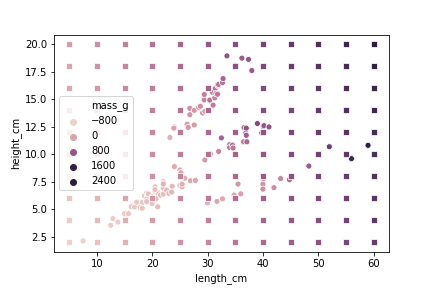
sns.scatterplot(x="length_cm",
                y="height_cm",
                data=prediction_data,
                hue="mass_g",
                legend=False,
                marker="s")

plt.show()

鱼的长度、高度与质量的散点图，并带有预测网格。

加入交互项

mdl_mass_vs_both_inter = ols("mass_g ~ length_cm * height_cm",
                             data=fish).fit()

print(mdl_mass_vs_both_inter.params)

Intercept              159.107480
length_cm                0.301426
height_cm              -78.125178
length_cm:height_cm      3.545435

含交互项的预测流程

length_cm = np.arange(5, 61, 5)
height_cm = np.arange(2, 21, 2)

p = product(length_cm, height_cm)

explanatory_data = pd.DataFrame(p,
                                columns=["length_cm",
                                         "height_cm"])

prediction_data = explanatory_data.assign(
  mass_g = mdl_mass_vs_both_inter.predict(explanatory_data))

绘制预测结果

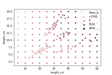
sns.scatterplot(x="length_cm",
           y="height_cm",
           data=fish,
           hue="mass_g")

sns.scatterplot(x="length_cm",
                y="height_cm",
                data=prediction_data,
                hue="mass_g",
                legend=False,
                marker="s")

plt.show()

鱼的长度、高度与质量的散点图，预测网格中包含交互项。

让我们来练习！

Python 中级回归：使用 statsmodels