比较不同插补技术的评估
在 Python 中处理缺失数据

Suraj Donthi
Deep Learning & Computer Vision Consultant
评估方法
- 插补用于提升模型表现。
- 选择使机器学习模型表现最佳的插补方式。
- 密度图展示数据分布。
- 检查插补偏差的优良指标。
拟合线性模型以获取统计摘要
import statsmodels.api as smdiabetes_cc = diabetes.dropna(how='any') X = sm.add_constant(diabetes_cc.iloc[:, :-1]) y = diabetes_cc['Class'] lm = sm.OLS(y, X).fit()
print(lm.summary())
Summary:                              OLS Regression Results
==============================================================================
Dep. Variable:                  Class   R-squared:                       0.346
Model:                            OLS   Adj. R-squared:                  0.332
Method:                 Least Squares   F-statistic:                     25.30
Date:                Wed, 10 Jul 2019   Prob (F-statistic):           2.65e-31
Time:                        15:03:19   Log-Likelihood:                -177.76
No. Observations:                 392   AIC:                             373.5
Df Residuals:                     383   BIC:                             409.3
Df Model:                           8
Covariance Type:            nonrobust
=====================================================================================
                        coef    std err          t      P>|t|      [0.025      0.975]
<hr />----------------------------------------------------------------------------------
const                -1.1027      0.144     -7.681      0.000      -1.385      -0.820
Pregnant              0.0130      0.008      1.549      0.122      -0.003       0.029
Glucose               0.0064      0.001      7.855      0.000       0.005       0.008
Diastolic_BP       5.465e-05      0.002      0.032      0.975      -0.003       0.003
Skin_Fold             0.0017      0.003      0.665      0.506      -0.003       0.007
Serum_Insulin        -0.0001      0.000     -0.603      0.547      -0.001       0.000
BMI                   0.0093      0.004      2.391      0.017       0.002       0.017
Diabetes_Pedigree     0.1572      0.058      2.708      0.007       0.043       0.271
Age                   0.0059      0.003      2.109      0.036       0.000       0.011
R-squared 与系数
lm.rsquared_adj
0.33210
lm.params
const               -1.102677
Pregnant             0.012953
Glucose              0.006409
Diastolic_BP         0.000055
Skin_Fold            0.001678
Serum_Insulin       -0.000123
BMI                  0.009325
Diabetes_Pedigree    0.157192
Age                  0.005878
dtype: float64
在不同插补的 DataFrame 上拟合线性模型
# Mean Imputation X = sm.add_constant(diabetes_mean_imputed.iloc[:, :-1]) y = diabetes['Class'] lm_mean = sm.OLS(y, X).fit()# KNN Imputation X = sm.add_constant(diabetes_knn_imputed.iloc[:, :-1]) lm_KNN = sm.OLS(y, X).fit()# MICE Imputation X = sm.add_constant(diabetes_mice_imputed.iloc[:, :-1]) lm_MICE = sm.OLS(y, X).fit()
比较不同插补的 R-squared
print(pd.DataFrame({'Complete': lm.rsquared_adj,
                          'Mean Imp.': lm_mean.rsquared_adj,
                          'KNN Imp.': lm_KNN.rsquared_adj,
                          'MICE Imp.': lm_MICE.rsquared_adj},
                         index=['R_squared_adj']))
                        Complete   Mean Imp.    KNN Imp.   MICE Imp.
R_squared_adj           0.332108    0.313781    0.316543    0.317679
注意:此处的度量仅适用于线性相关。请使用能反映数据特性的度量。
比较不同插补的系数
print(pd.DataFrame({'Complete': lm.params,
                          'Mean Imp.': lm_mean.params,
                          'KNN Imp.': lm_KNN.params,
                          'MICE Imp.': lm_MICE.params}))
                        Complete   Mean Imp.    KNN Imp.   MICE Imp.
const                  -1.102677   -1.024005   -1.028035   -1.050023
Pregnant                0.012953    0.020693    0.020047    0.020295
Glucose                 0.006409    0.006467    0.006614    0.006871
Diastolic_BP            0.000055   -0.001137   -0.001196   -0.001317
Skin_Fold               0.001678    0.000193    0.001626    0.000807
Serum_Insulin          -0.000123   -0.000090   -0.000147   -0.000227
BMI                     0.009325    0.014376    0.013239    0.014203
Diabetes_Pedigree       0.157192    0.129282    0.128038    0.129056
Age                     0.005878    0.002092    0.002046    0.002097
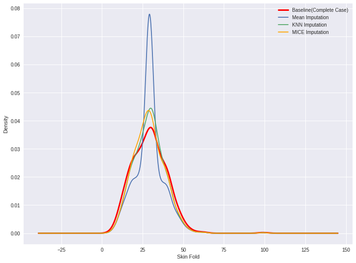
比较密度图
diabetes_cc['Skin_Fold'].plot(kind='kde', c='red', linewidth=3)
diabetes_mean_imputed['Skin_Fold'].plot(kind='kde')
diabetes_knn_imputed['Skin_Fold'].plot(kind='kde')
diabetes_mice_imputed['Skin_Fold'].plot(kind='kde')

labels = ['Baseline (Complete Case)', 'Mean Imputation', 'KNN Imputation',
          'MICE Imputation']
plt.legend(labels)
plt.xlabel('Skin Fold')
比较密度图
总结
- 使用 statsmodels 包的线性模型
- 比较系数与标准误
- 比较密度图
Passons à la pratique !
在 Python 中处理缺失数据

