结果可视化

使用 R 中的 Bioconductor 进行 RNA-Seq 分析

Mary Piper

Bioinformatics Consultant and Trainer

结果可视化 - 表达热图

# Subset normalized counts to significant genes 
sig_norm_counts_wt <- normalized_counts_wt[wt_res_sig$ensgene, ]

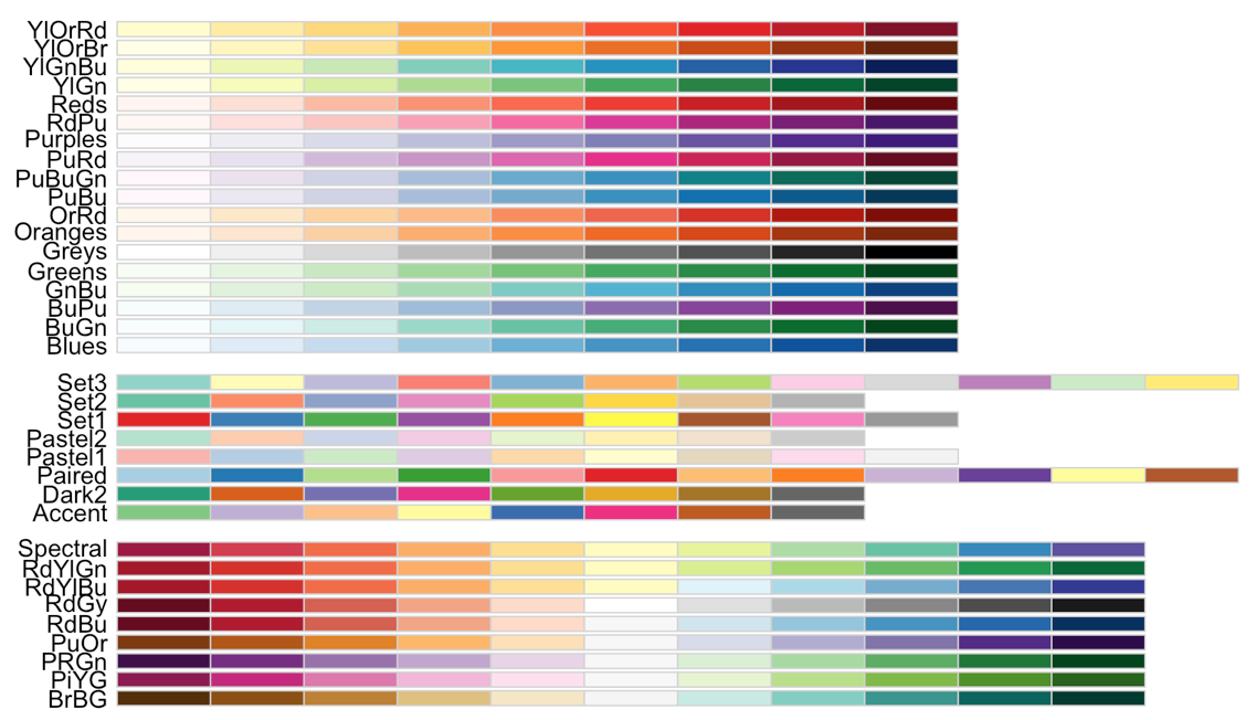
# Choose a color palette from RColorBrewer library(RColorBrewer) heat_colors <- brewer.pal(6, "YlOrRd")
display.brewer.all()

调色板

使用 R 中的 Bioconductor 进行 RNA-Seq 分析

结果可视化 - 表达热图

# Run pheatmap
pheatmap(sig_norm_counts_wt, 
         color = heat_colors, 
         cluster_rows = T, 
         show_rownames = F,
         annotation = select(wt_metadata, condition), 
         scale = "row")
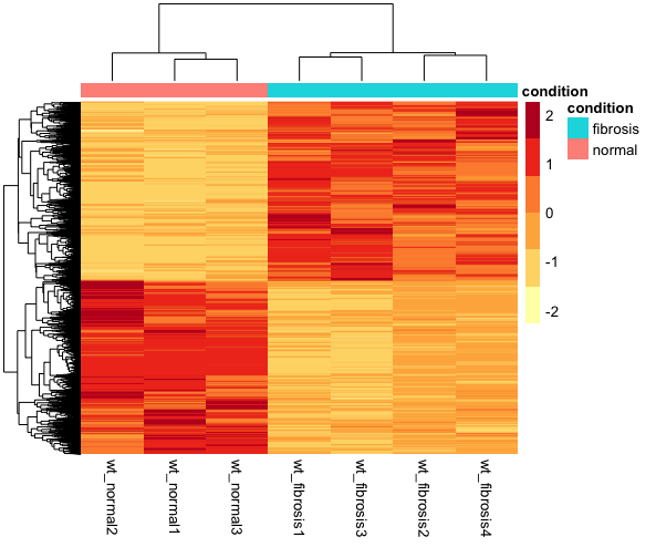
表达热图

使用 R 中的 Bioconductor 进行 RNA-Seq 分析

结果可视化 - 火山图

# Obtain logical vector regarding whether padj values are less than 0.05 
wt_res_all <- wt_res_all %>%
              rownames_to_column(var = "ensgene") %>%
              mutate(threshold = padj < 0.05)

# Volcano plot ggplot(wt_res_all) + geom_point(aes(x = log2FoldChange, y = -log10(padj), color = threshold)) + xlab("log2 fold change") + ylab("-log10 adjusted p-value") + theme(legend.position = "none", plot.title = element_text(size = rel(1.5), hjust = 0.5), axis.title = element_text(size = rel(1.25)))
使用 R 中的 Bioconductor 进行 RNA-Seq 分析
ggplot(wt_res_all) +
        geom_point(aes(x = log2FoldChange, y = -log10(padj), color = threshold)) +
        xlab("log2 fold change") + 
        ylab("-log10 adjusted p-value") +
        ylim=c(0, 15) +
        theme(legend.position = "none",
              plot.title = element_text(size = rel(1.5), hjust = 0.5),
              axis.title = element_text(size = rel(1.25)))
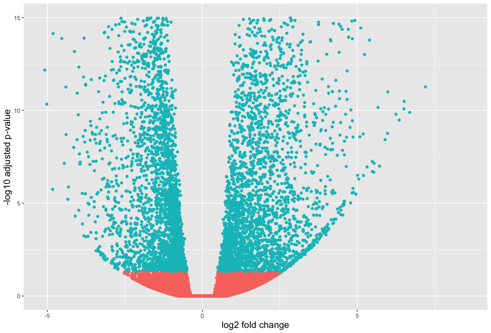
火山图(放大)

使用 R 中的 Bioconductor 进行 RNA-Seq 分析

结果可视化 - 表达图

显著结果:

显著结果

显著基因的标准化计数:

显著基因的标准化计数

使用 R 中的 Bioconductor 进行 RNA-Seq 分析

结果可视化 - 表达图

top_20 <- data.frame(sig_norm_counts_wt)[1:20, ] %>%
        rownames_to_column(var = "ensgene")

top_20 <- gather(top_20, key = "samplename", value = "normalized_counts", 2:8)
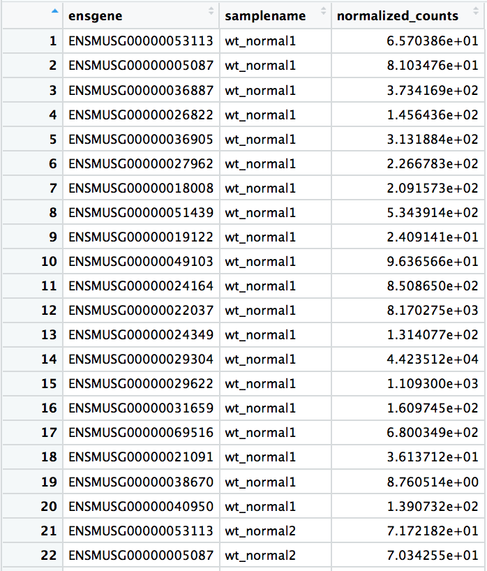
收集后的标准化计数

使用 R 中的 Bioconductor 进行 RNA-Seq 分析

结果可视化 - 表达图

top_20 <- inner_join(top_20,
                     rownames_to_column(wt_metadata, var = "samplename"),
                     by = "samplename")
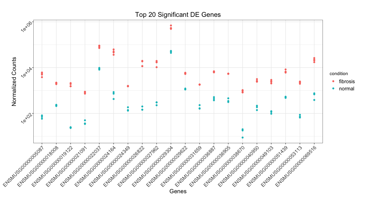
ggplot(top_20) +
        geom_point(aes(x = ensgene, y = normalized_counts, color = condition)) +
        scale_y_log10() +
        xlab("Genes") +
        ylab("Normalized Counts") +
        ggtitle("Top 20 Significant DE Genes") +
        theme_bw() +
        theme(axis.text.x = element_text(angle = 45, hjust = 1)) +
        theme(plot.title = element_text(hjust = 0.5))
使用 R 中的 Bioconductor 进行 RNA-Seq 分析

前20表达图

使用 R 中的 Bioconductor 进行 RNA-Seq 分析

Passons à la pratique !

使用 R 中的 Bioconductor 进行 RNA-Seq 分析

Preparing Video For Download...