R 中的分类数据推断
Andrew Bray
Assistant Professor of Statistics at Reed College
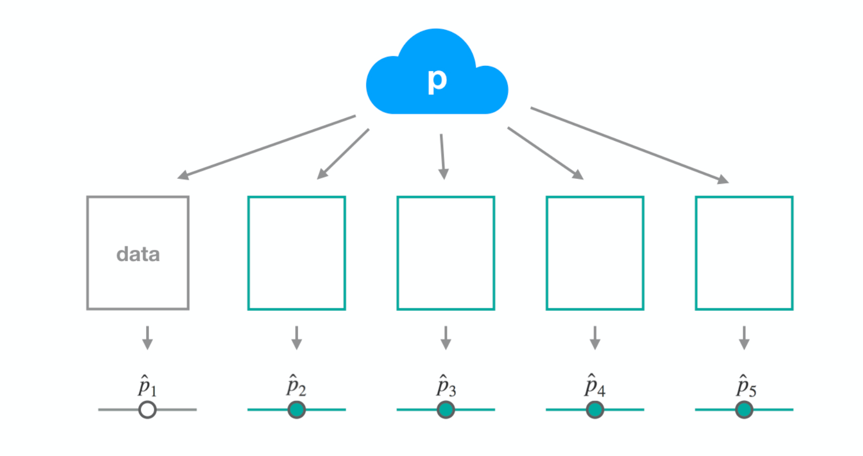
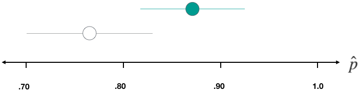
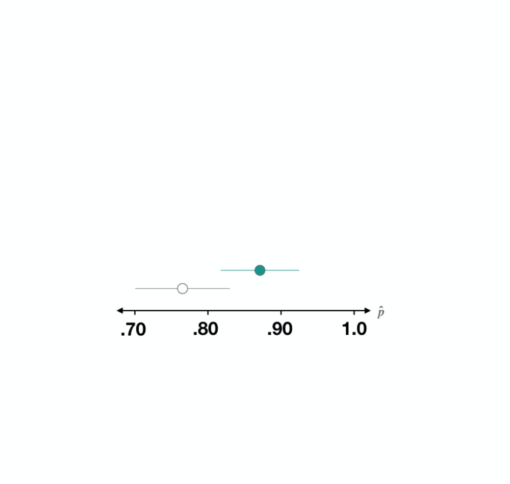
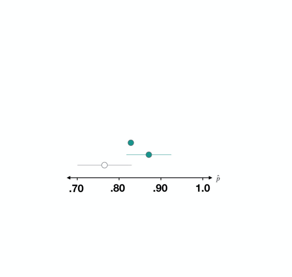
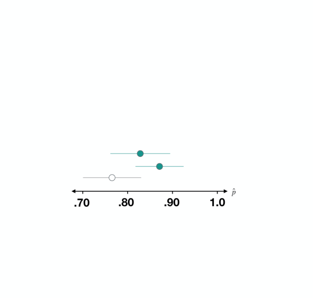
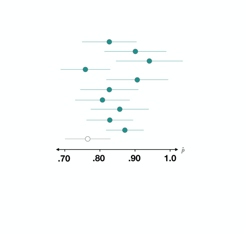
结论:美国人真正的快乐比例在 0.705 与 0.841 之间。
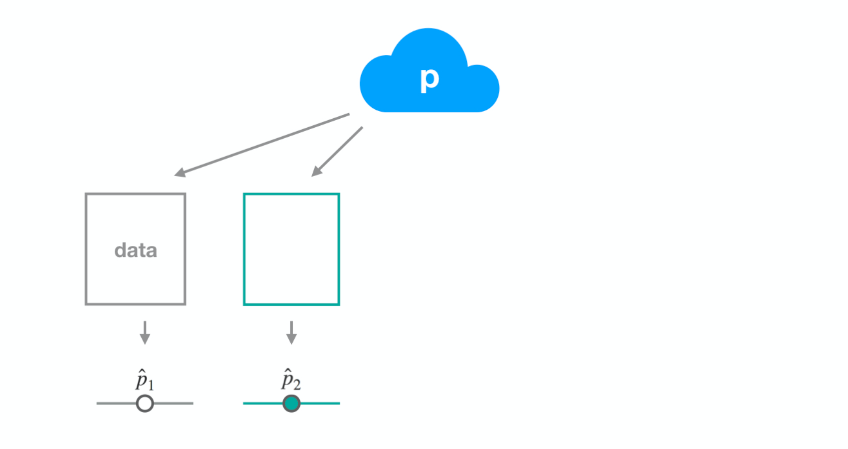
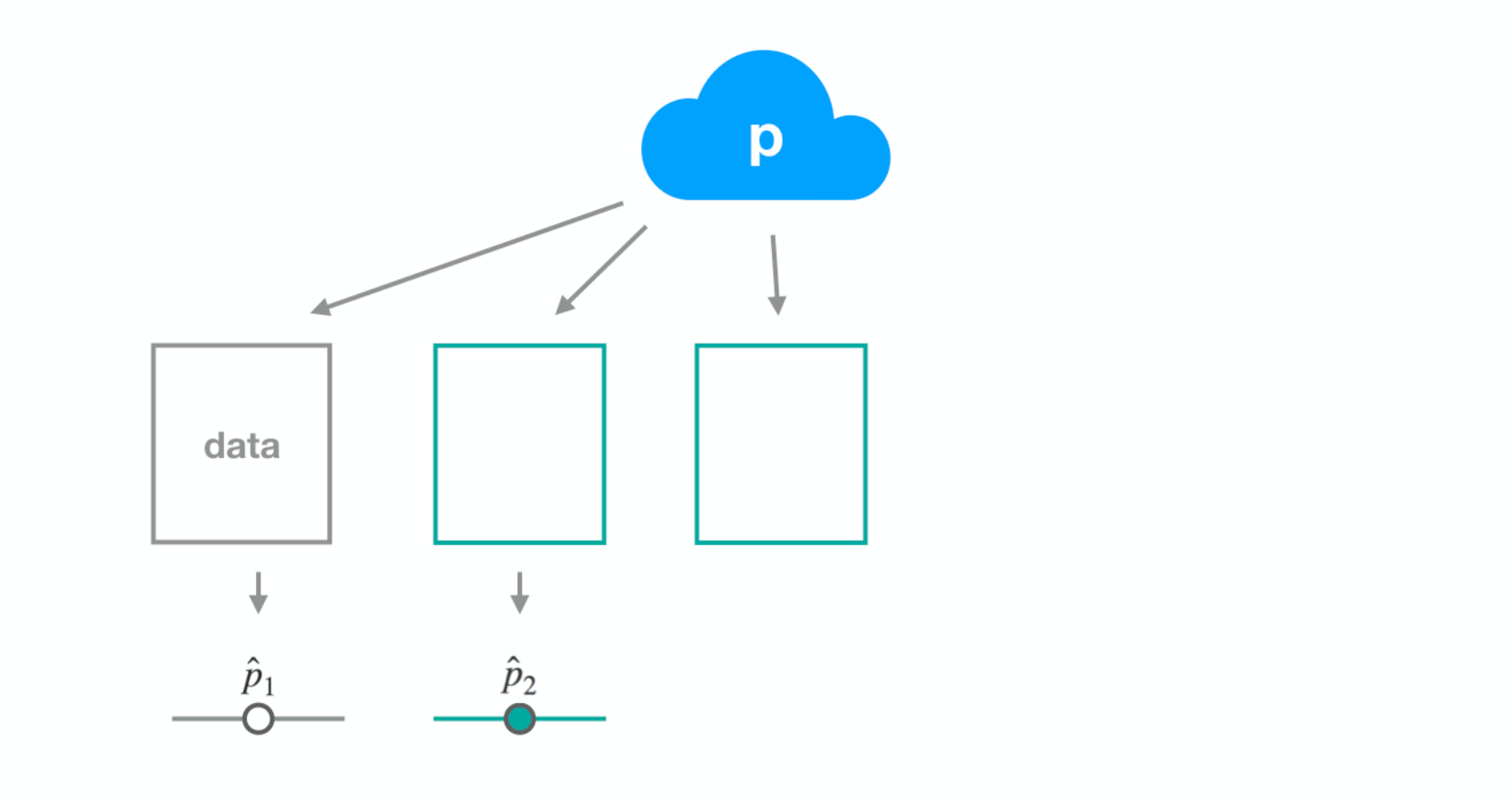
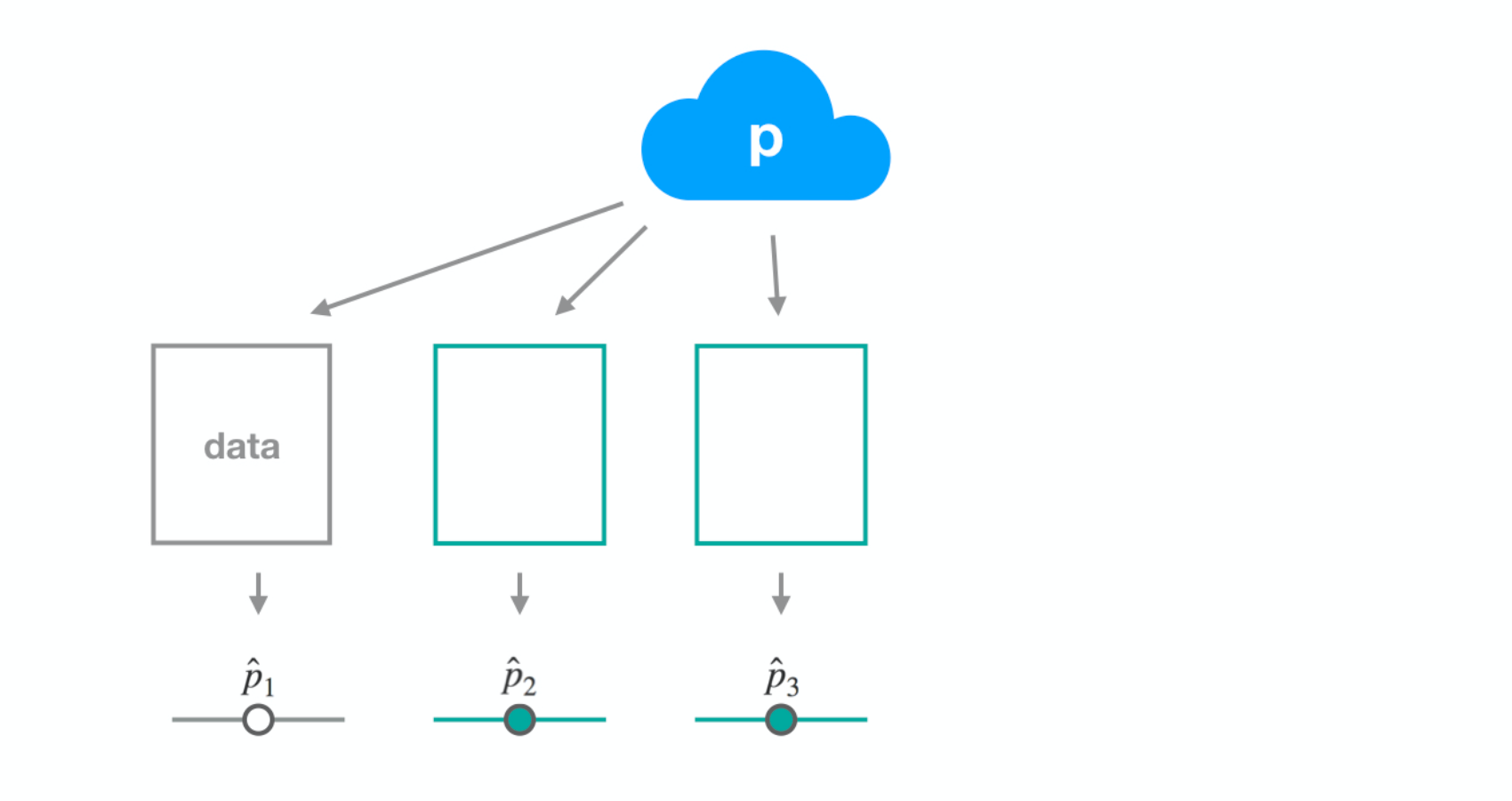
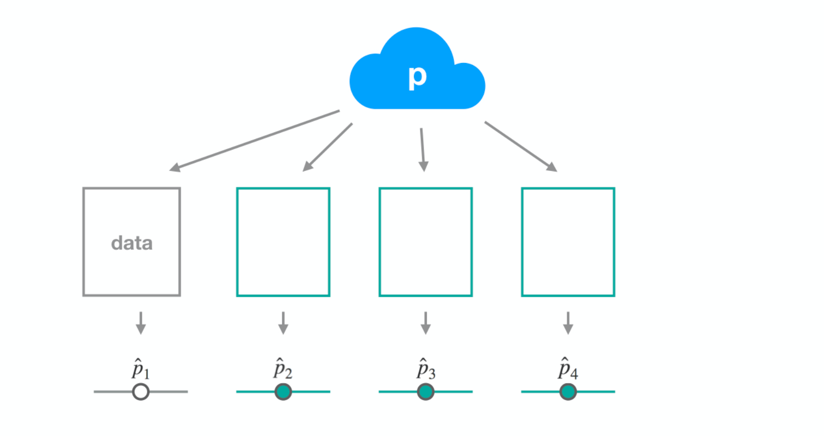
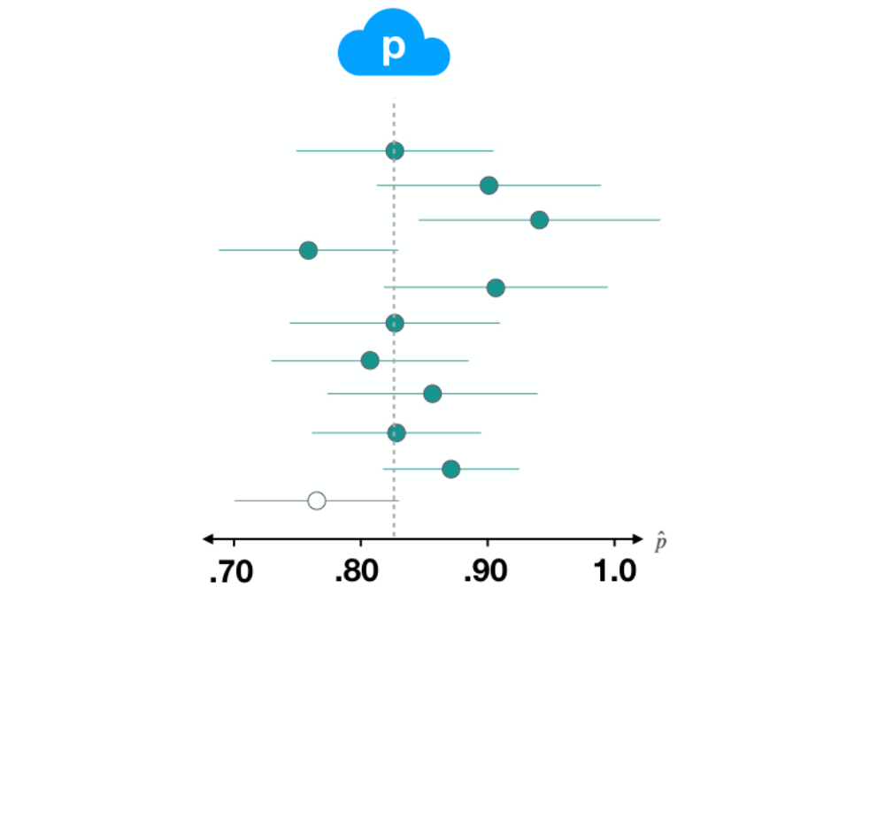
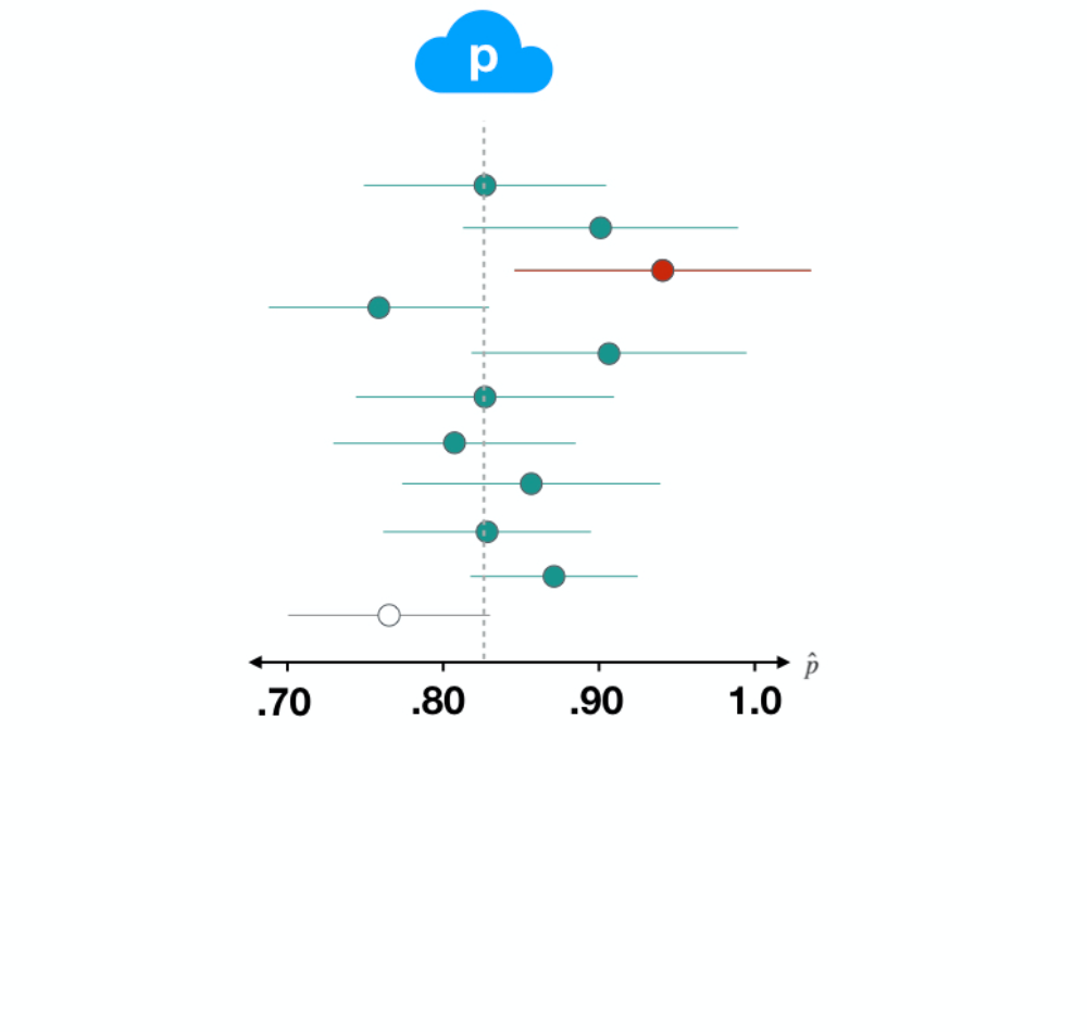
我们所说的"有把握"是什么意思?
ds1 <- filter(gss, year == 2016)

p_hat <- ds1 %>%
  summarize(mean(happy == "HAPPY")) %>%
  pull()

SE <- ds1 %>%
  specify(response = happy,
          success = "HAPPY") %>%
  generate(reps = 500,
           type = "bootstrap") %>%
  calculate(stat = "prop") %>%
  summarize(sd(stat)) %>%
  pull()

c(p_hat - 2 * SE, p_hat + 2 * SE)
ds1 <- filter(gss, year == 2016)
p_hat <- ds1 %>% summarize(mean(happy == "HAPPY")) %>% pull()
SE <- ds1 %>% specify(response = happy, success = "HAPPY") %>% generate(reps = 500, type = "bootstrap") %>% calculate(stat = "prop") %>% summarize(sd(stat)) %>% pull()
c(p_hat - 2 * SE, p_hat + 2 * SE)
0.7073114 0.8393553
ds2 <- filter(gss, year == 2014)

p_hat <- ds1 %>%
  summarize(mean(happy == "HAPPY")) %>%
  pull()

SE <- ds1 %>%
  specify(response = happy,
          success = "HAPPY") %>%
  generate(reps = 500,
           type = "bootstrap") %>%
  calculate(stat = "prop") %>%
  summarize(sd(stat)) %>%
  pull()

c(p_hat - 2 * SE, p_hat + 2 * SE)
ds2 <- filter(gss, year == 2014)
0.8348831 0.9384503
ds3 <- filter(gss, year == 2012)

p_hat <- ds1 %>%
  summarize(mean(happy == "HAPPY")) %>%
  pull()

SE <- ds1 %>%
  specify(response = happy,
          success = "HAPPY") %>%
  generate(reps = 500,
           type = "bootstrap") %>%
  calculate(stat = "prop") %>%
  summarize(sd(stat)) %>%
  pull()

c(p_hat - 2 * SE, p_hat + 2 * SE)
ds3 <- filter(gss, year == 2012)
0.7626359 0.8906974
ds3 <- filter(gss, year == 2012)
p_hat <- ds3 %>%
  summarize(mean(happy == "HAPPY")) %>%
  pull()
SE <- ds3 %>%
  specify(response = happy,
          success = "HAPPY") %>%
  generate(reps = 500,
           type = "bootstrap") %>%
  calculate(stat = "prop") %>%
  summarize(sd(stat)) %>%
  pull()

c(p_hat - 2 * SE, p_hat + 2 * SE)
ds3 <- filter(gss, year == 2012) p_hat <- ds3 %>% summarize(mean(happy == "HAPPY")) %>% pull() SE <- ds3 %>% specify(response = happy, success = "HAPPY") %>% generate(reps = 500, type = "bootstrap") %>% calculate(stat = "prop") %>% summarize(sd(stat)) %>% pull()
解读:"我们有 95% 的把握认为,美国人真实的快乐比例在 0.705 与 0.841 之间。"
区间宽度受以下因素影响
n
p