可视化数据分布

在 Python 中导入与管理金融数据

Stefan Jansen

Instructor

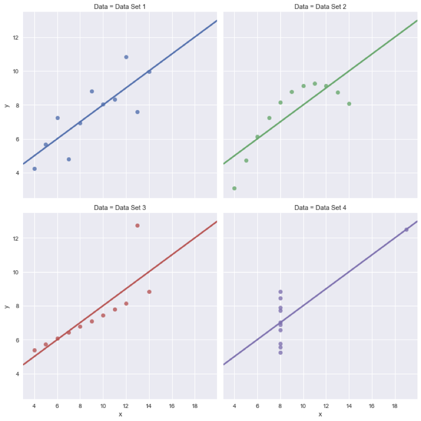
务必查看你的数据！

相同指标可能代表非常不同的数据

务必查看.png

认识 seaborn 图

许多美观且有洞见的统计图
基于 matplotlib
瑞士军刀：seaborn.distplot()
- 直方图
- 核密度估计（KDE）
- 地毯图

10 年期国债：趋势与分布

ty10 = web.DataReader('DGS10', 'fred', date(1962, 1, 1))
ty10.info()

DatetimeIndex: 15754 entries, 1962-01-02 to 2022-05-20
Data columns (total 1 columns):
 #   Column  Non-Null Count  Dtype  
 --  ------  --------------  -----  
 0   DGS10   15083 non-null  float64

ty10.describe()

              DGS10
mean       6.291073
std        2.851161
min        1.370000
25%        4.190000
50%        6.040000
...

10 年期国债：时间序列趋势

ty10.dropna(inplace=True) # Avoid creation of copy

ty10.plot(title='10-year Treasury'); plt.tight_layout()

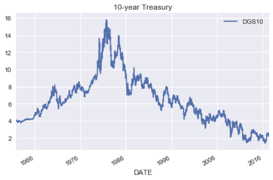
10年期国债收益率.png

10 年期国债：历史分布

import seaborn as sns
sns.distplot(ty10)

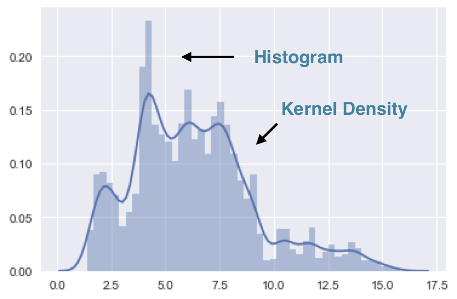
10年期直方图.png

10 年期国债：趋势与分布

ax = sns.distplot(ty10)
ax.axvline(ty10['DGS10'].median(), color='black', ls='--')

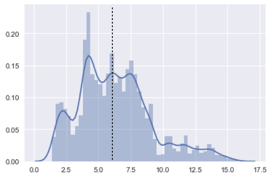
10年期收益率密度.png

¡Vamos a practicar!

在 Python 中导入与管理金融数据