回归分析中的主成分

用 R 进行市场营销分析的机器学习

Verena Pflieger

Data Scientist at INWT Statistics

回归分析中的主成分 I

mod1 <- lm(customerSatis ~ ., dataCustomers)

library(car)
vif(mod1)

      nOrders       nItemsOrdered          nItemsSold        salesOrdered 
    29.482287           24.437448           10.390998            5.134720 
    salesSold         returnRatio       shareOwnBrand           shareSale 
     9.685617           23.778800            1.571607            1.178773 
 shareVoucher          crDuration monetaryReturnRatio  meanDaysBetwOrders 
     1.213011            1.757509           10.632243            1.698369 
salesPerOrder        salesPerItem       itemsPerOrder   itemsSoldPerOrder 
     6.563474            4.557981            4.821610           15.949072

# Create dataframe with customer satisfaction and first 6 components
dataCustComponents <- cbind(dataCustomers[, "customerSatis"], 
                            pcaCust$x[,1:6]) %>%
  as.data.frame
mod2 <- lm(customerSatis ~ ., dataCustComponents)
vif(mod2)

PC1 PC2 PC3 PC4 PC5 PC6 
  1   1   1   1   1   1

summary(mod1)$adj.r.squared

0.8678583

summary(mod2)$adj.r.squared

0.7123822

summary(mod2)

Call:
lm(formula = customerSatis ~ ., data = dataCustComponents)
Residuals:
    Min      1Q  Median      3Q     Max 
-3.9279 -0.2411  0.0179  0.2865  1.4972 
Coefficients:
             Estimate Std. Error t value Pr(>|t|)    
(Intercept)  2.985945   0.014039 212.682  < 2e-16 ***
PC1         -0.175434   0.006704 -26.167  < 2e-16 ***
PC2          0.296659   0.007643  38.815  < 2e-16 ***
PC3         -0.012816   0.010838  -1.182    0.237    
PC4         -0.116651   0.011665 -10.000  < 2e-16 ***
PC5          0.101963   0.012508   8.152 1.09e-15 ***
PC6          0.126677   0.013072   9.691  < 2e-16 ***
- - -
Signif. codes:  0 '***' 0.001 '**' 0.01 '*' 0.05 '.' 0.1 ' ' 1
Residual standard error: 0.4415 on 982 degrees of freedom
Multiple R-squared:  0.7141,    Adjusted R-squared:  0.7124 
F-statistic: 408.9 on 6 and 982 DF,  p-value: < 2.2e-16

	关于 PCA 的收获
你已学会…	在不丢失太多信息的情况下减少变量数量
	在做 PCA 前应对变量标准化
	如何确定相关成分的数量
	如何解释选定的成分

	来自模型的收获
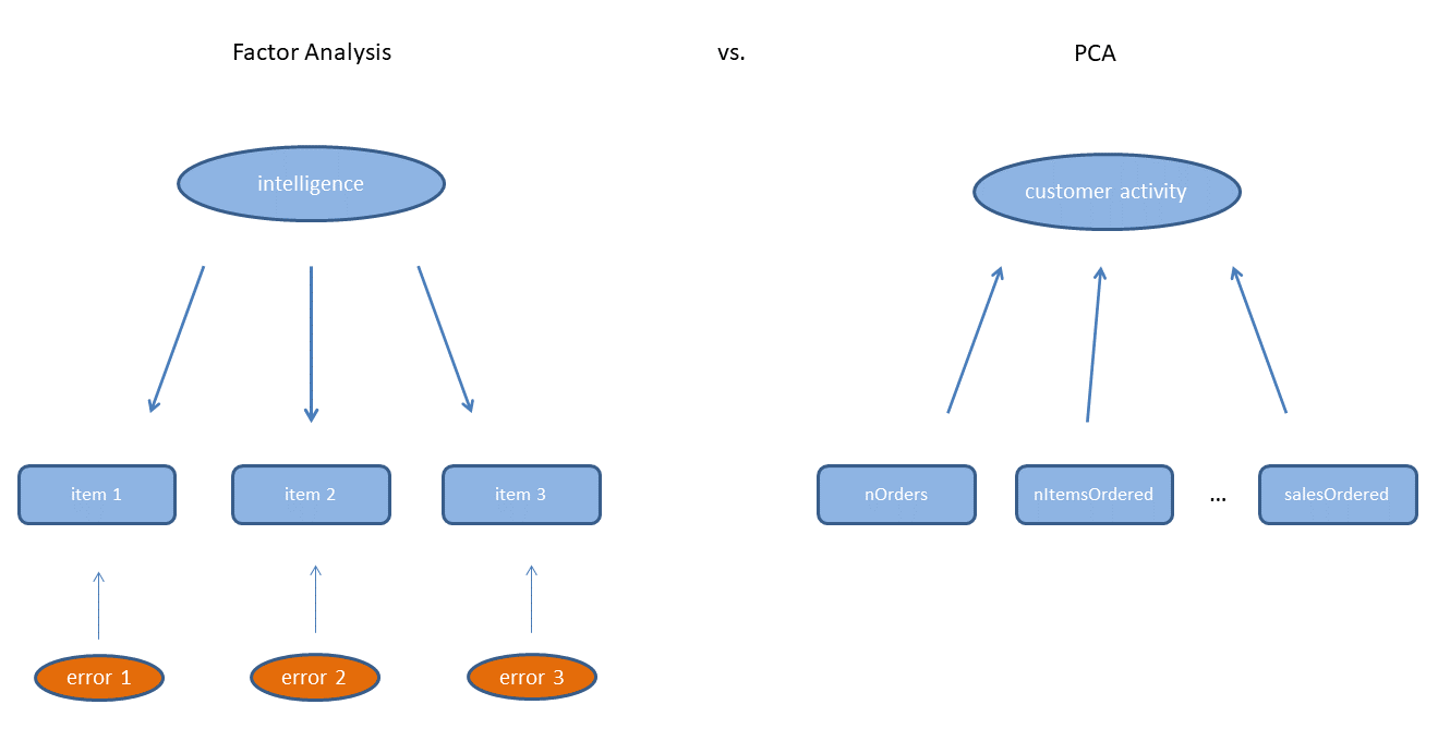
你已学会…	原始变量可归纳为 6 个成分，如客户活跃度、退货行为与品牌认知等
	用前 6 个成分解释客户满意度会降低解释方差，但可解决多重共线性问题

Passons à la pratique !

用 R 进行市场营销分析的机器学习