什么是特征工程？

R 中的特征工程

Jorge Zazueta

Research Professor and Head of the Modeling Group at the School of Economics, UASLP

什么是特征工程？

特征工程是关于

创建，
变换，
提取，以及
选择

变量，以提升模型性能与可解释性。

物体高度随时间变化

# A tibble: 100 × 2
    time height
   <dbl>  <dbl>
 1 0       0   
 2 0.101   3.85
 3 0.202  17.7 
 4 0.303  15.1 
 5 0.404  20.0 
 6 0.505  32.6 
 7 0.606  30.8 
 8 0.707  26.6 
 9 0.808  33.8 
10 0.909  39.2 
# ... with 90 more rows
# ℹ Use `print(n = ...)` to see more rows

为何进行特征工程？

我们先建立一个高度的简单回归模型

lr_height <- lm(height ~ time,
                data = height)

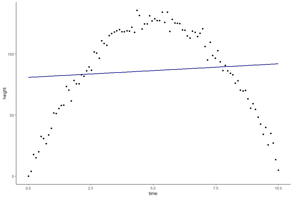
并绘图以目测其准确性。

df <- height %>% 
bind_cols(lr_pred = predict(lr_height))

df %>%
  ggplot(aes(x = time, y = height)) +
  geom_point() +
  geom_line(aes(y = lr_pred), 
            color = "blue", lwd = .75)+
    theme_classic()

该模型明显无法刻画数据！

高度与时间的线性回归。

高度与时间的线性回归，显示拟合不足。

使用 mutate()

物体高度遵循抛物线轨迹，公式如下：

$y(t) = y_0 + v_0t - \frac{g}{2}t^2$。

其中，$y$ 为时刻 $t$ 的高度，$y_0$、$v_0$、$g$ 分别为初始高度、初速度与重力加速度。

据此可拟合模型，使高度依赖于时间与时间的平方。

mutate() 以数据框为首个参数，并接收要添加的新变量定义。

df_2 <- df %>% mutate(time_2 = time^2)

# A tibble: 100 × 4
    time height lr_pred time_2
   <dbl>  <dbl>   <dbl>  <dbl>
 1 0       0       80.8 0     
 2 0.101   3.85    80.9 0.0102
 3 0.202  17.7     81.0 0.0408
 4 0.303  15.1     81.1 0.0918

用工程化特征进行预测

我们基于新特征与原始特征一起再建一个回归模型。

lr_height_2 <- 
lm(height ~ time + time_2, data = df_2)

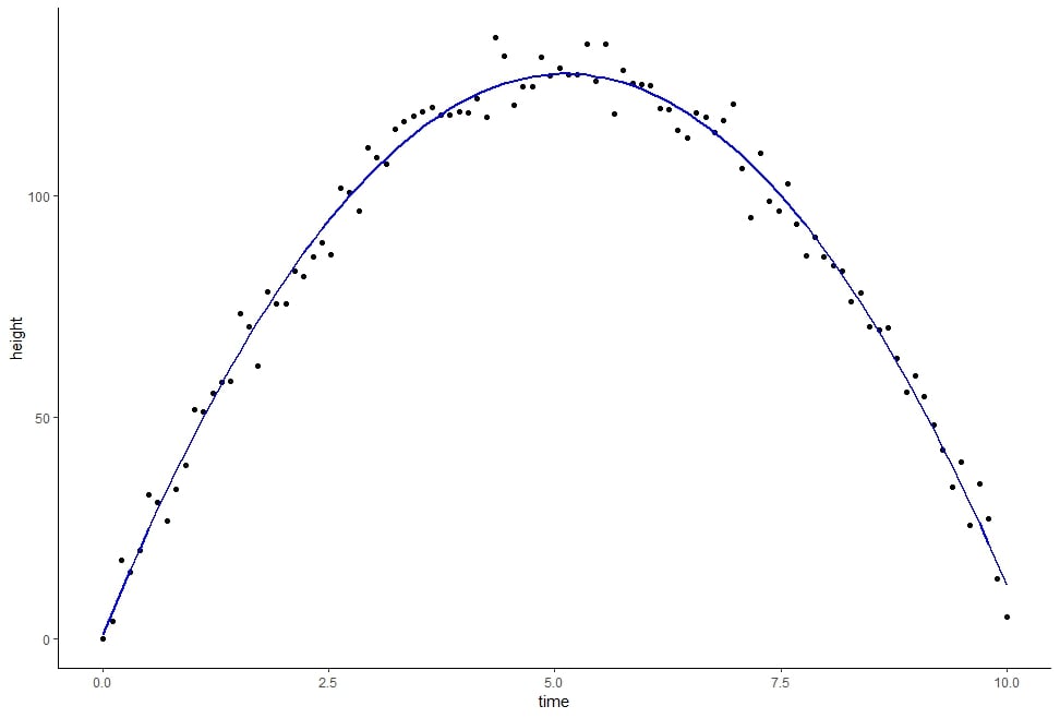
并绘制新的预测。

df_2 <- df_2 %>%
    bind_cols(lr2_pred = predict(lr_height_2))
df_2 %>%
  ggplot(aes(x = time, y = height)) +
  geom_point() +
  geom_line(aes(y = lr2_pred), 
      col = "blue", lwd = .75) +
  theme_classic()

无需更换模型就有显著提升。

高度与 time 与 time_2 的关系

让我们来练习！

R 中的特征工程