建模数据

在 R 中使用 limma 进行差异表达分析

John Blischak

Instructor

准备分析

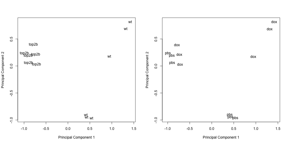
# Plot principal components labeled by genotype
plotMDS(eset, labels = pData(eset)[, "genotype"], gene.selection = "common")
# Plot principal components labeled by treatment
plotMDS(eset, labels = pData(eset)[, "treatment"], gene.selection = "common")

差异表达分析步骤

用 model.matrix 构建设计矩阵
用 makeContrasts 构建对比矩阵
用 lmFit、contrasts.fit 和 eBayes 检验对比

阿霉素研究的组均值模型

$$ Y = \beta_1 X_1 + \beta_2 X_2 + \beta_3 X_3 + \beta_4 X_4 + \epsilon $$

$\beta_1$：top2b 小鼠用 dox 处理的平均表达
$\beta_2$：top2b 用 pbs 处理的平均表达
$\beta_3$：wt 小鼠用 dox 处理的平均表达
$\beta_4$：wt 小鼠用 pbs 处理的平均表达

阿霉素研究的对比

	$\beta_1$	$\beta_2$	$\beta_3$	$\beta_4$
`genotype`	top2b	top2b	wt	wt
`treatment`	dox	pbs	dox	pbs

Response of wild type mice to dox treatment: $\beta_3 - \beta_4 = 0$
Response of Top2b null mice to dox treatment: $\beta_1 - \beta_2 = 0$
Differences between Top2b null and wild type mice in response to dox treatment: $(\beta_1 - \beta_2) - (\beta_3 - \beta_4) = 0$

阿霉素研究的检验

用 lmFit 拟合模型系数
用 contrasts.fit 拟合对比
用 eBayes 计算 t 统计量

# Summarize results
results <- decideTests(fit2)
summary(results)

# Create a Venn diagram
vennDiagram(results)

开始练习！

在 R 中使用 limma 进行差异表达分析