分类数据：分析与可视化

面向 SAS 用户的 R

Melinda Higgins, PhD

Research Professor/Senior Biostatistician Emory University

合并类别

# Use table() inside with() for bmicat
daviskeep %>% with(table(bmicat))

bmicat
1. underwt/norm       2. overwt        3. obese
            161              35               3

添加重编码变量 bmigt25

# Add one more categorical variable bmigt25
daviskeep <- daviskeep %>%
  mutate(bmigt25 = ifelse(bmi > 25,
                          "2. overwt/obese",
                          "1. underwt/norm"))

# View frequencies for bmigt25 categories
daviskeep %>% with(table(bmigt25))

bmigt25
1. underwt/norm 2. overwt/obese
            161              38

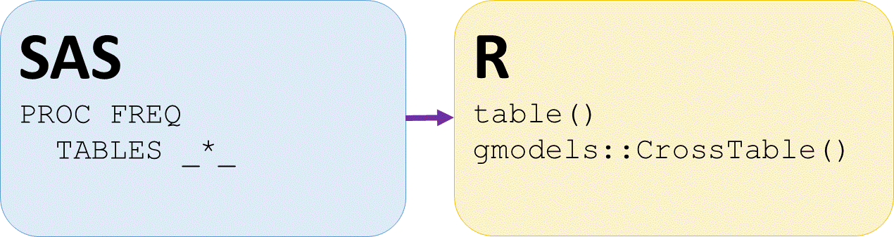
SAS 与 R 的列联表

SAS 的 PROC FREQ 与 R 的 table 函数及 gmodels 包的 CrossTable

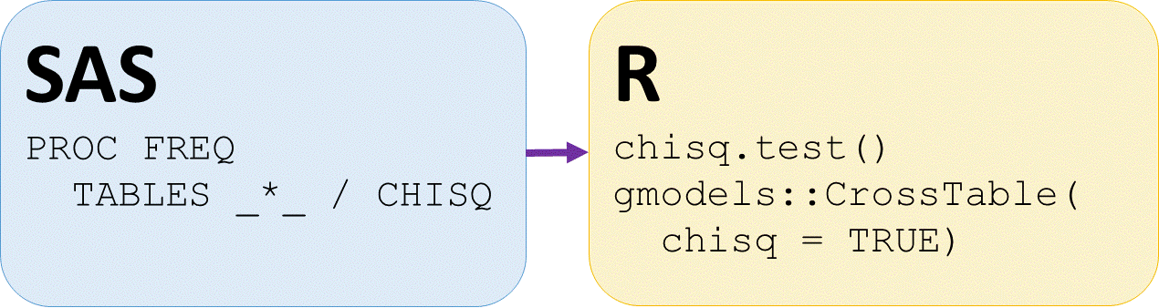
SAS 与 R 的卡方检验

SAS PROC FREQ 与 R 代码：chisq.test 及 gmodels 包 CrossTable 选项

列联表与卡方检验

# Save table output of bmigt25 by sex
tablebmisex <- daviskeep %>%
  with(table(bmigt25, sex))
tablebmisex

# Use table object to run chisq.test
chisq.test(tablebmisex)

                 sex
bmigt25             F   M
  1. underwt/norm 107  54
  2. overwt/obese   4  34

Pearson's Chi-squared test with Yates'
continuity correction

data:  tablebmisex
X-squared = 36.759, df = 1, p-value = 1.336e-09

使用 gmodels 包进行卡方检验

# Load gmodel package
library(gmodels)

# Run gmodels::CrossTabs, show column %s and expected values
daviskeep %>%
  with(gmodels::CrossTable(bmigt25, sex,
                           chisq = TRUE,
                           prop.r = FALSE,
                           prop.t = FALSE,
                           prop.chisq = FALSE,
                           expected = TRUE))

CrossTable 输出 - 第 1 部分

   Cell Contents
|-------------------------|
|                       N |
|              Expected N |
|           N / Col Total |
|-------------------------|

Total Observations in Table:  199

                | sex
        bmigt25 |         F |         M | Row Total |
----------------|-----------|-----------|-----------|
1. underwt/norm |       107 |        54 |       161 |
                |    89.804 |    71.196 |           |
                |     0.964 |     0.614 |           |
----------------|-----------|-----------|-----------|
2. overwt/obese |         4 |        34 |        38 |
                |    21.196 |    16.804 |           |
                |     0.036 |     0.386 |           |
----------------|-----------|-----------|-----------|
   Column Total |       111 |        88 |       199 |
                |     0.558 |     0.442 |           |
----------------|-----------|-----------|-----------|

CrossTable 输出 - 第 2 部分

gmodels::CrossTable() 输出 - 续

Statistics for All Table Factors

Pearson's Chi-squared test
------------------------------------------------------------
Chi^2 =  38.99402     d.f. =  1     p =  4.251066e-10

Pearson's Chi-squared test with Yates' continuity correction
------------------------------------------------------------
Chi^2 =  36.75936     d.f. =  1     p =  1.336475e-09

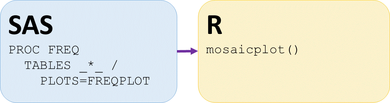
SAS 与 R 的马赛克图

SAS 的 PROC FREQ 表语句 freqplot 选项与 R 的 mosaicplot 函数

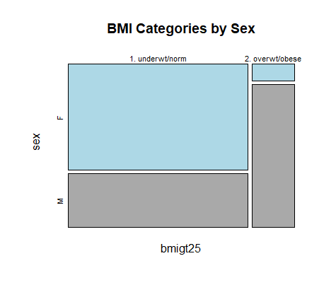
二维分类比例的马赛克图

# Make mosaicplot of bmigt25 by sex
mosaicplot(bmigt25 ~ sex,
           data = daviskeep,
           color = c("light blue",
                     "dark grey"),
           main =
             "BMI Categories by Sex")

daviskeep 数据集中 bmigt25 与 sex 的马赛克图

一起探索鲍鱼数据的分类关联！

面向 SAS 用户的 R