Inspecția vizuală a datelor

Feature Engineering cu PySpark

John Hogue

Lead Data Scientist, General Mills

Statistici descriptive cu DataFrame.describe()

df.describe(['LISTPRICE']).show()
+-------+------------------+
|summary|         LISTPRICE|
+-------+------------------+
|  count|              5000|
|   mean|        263419.365|
| stddev|143944.10818036905|
|    min|            100000|
|    max|             99999|
+-------+------------------+
Feature Engineering cu PySpark

Numeroase funcții descriptive sunt deja disponibile

  • Medie
    • pyspark.sql.functions.mean(col)
  • Asimetrie
    • pyspark.sql.functions.skewness(col)
  • Minim
    • pyspark.sql.functions.min(col)
  • Covarianță
    • cov(col1, col2)
  • Corelație
    • corr(col1, col2)
Feature Engineering cu PySpark

Exemplu cu mean()

  • mean(col)
  • Funcție de agregare: returnează media valorilor dintr-un grup.
df.agg({'SALESCLOSEPRICE': 'mean'}).collect()
[Row(avg(SALESCLOSEPRICE)=262804.4668)]
Feature Engineering cu PySpark

Exemplu cu cov()

  • cov(col1, col2)
  • Parametri:
    • col1 – prima coloană
    • col2 – a doua coloană
df.cov('SALESCLOSEPRICE', 'YEARBUILT')
1281910.3840634783
Feature Engineering cu PySpark

seaborn: vizualizare statistică a datelor
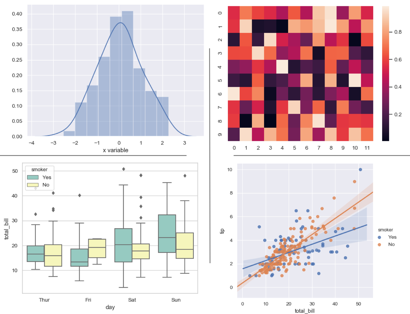
Seaborn

Feature Engineering cu PySpark

Note despre reprezentarea grafică

Reprezentarea grafică a DataFrame-urilor PySpark cu biblioteci precum Seaborn necesită conversie în Pandas

ATENȚIE: Eșantionați DataFrame-urile PySpark înainte de conversia în Pandas!

  • sample(withReplacement, fraction, seed=None)
    • withReplacement permite repetițiile în eșantion
    • fraction % din înregistrări de păstrat
    • seed sămânță aleatoare pentru reproductibilitate
# Sample 50% of the PySpark DataFrame and count rows
df.sample(False, 0.5, 42).count()
2504
Feature Engineering cu PySpark

Pregătire pentru reprezentarea distribuției

Seaborn distplot()

  • seaborn.distplot(a)
  • a : Series, array 1D sau listă. Date observate.
# Import your favorite visualization library
import seaborn as sns

# Sample the dataframe sample_df = df.select(['SALESCLOSEPRICE']).sample(False, 0.5, 42)
# Convert the sample to a Pandas DataFrame pandas_df = sample_df.toPandas()
# Plot it sns.distplot(pandas_df)
Feature Engineering cu PySpark

Distribuția prețului de închidere a vânzărilor
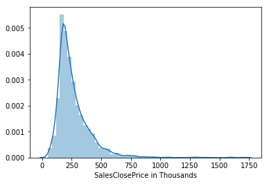
Grafic de distribuție

Feature Engineering cu PySpark

Reprezentarea relațiilor

Seaborn lmplot()

  • seaborn.lmplot(x, y, data)
  • x, y : șiruri de caractere, variabile de intrare; trebuie să fie nume de coloane din date.
  • data : DataFrame Pandas
# Import your favorite visualization library
import seaborn as sns

# Select columns s_df = df.select(['SALESCLOSEPRICE', 'SQFTABOVEGROUND']) # Sample dataframe s_df = s_df.sample(False, 0.5, 42)
# Convert to Pandas DataFrame pandas_df = s_df.toPandas()
# Plot it sns.lmplot(x='SQFTABOVEGROUND', y='SALESCLOSEPRICE', data=pandas_df)
Feature Engineering cu PySpark

Model liniar între SQFT deasupra solului și prețul de vânzare
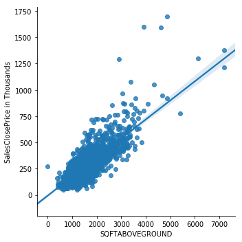
Grafic model liniar

Feature Engineering cu PySpark

Să exersăm!

Feature Engineering cu PySpark

Preparing Video For Download...