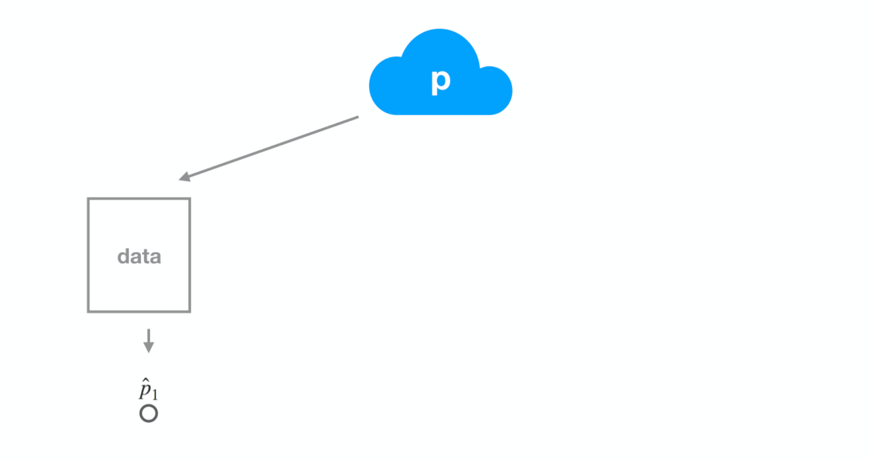
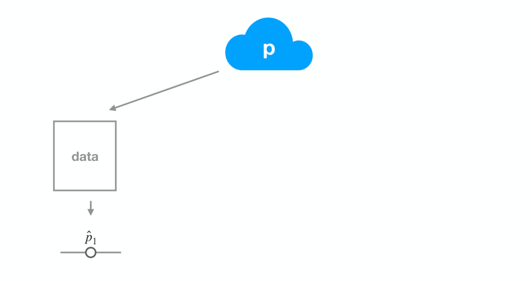
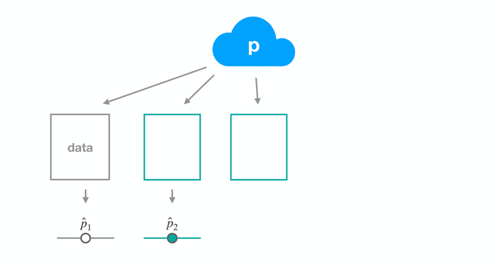
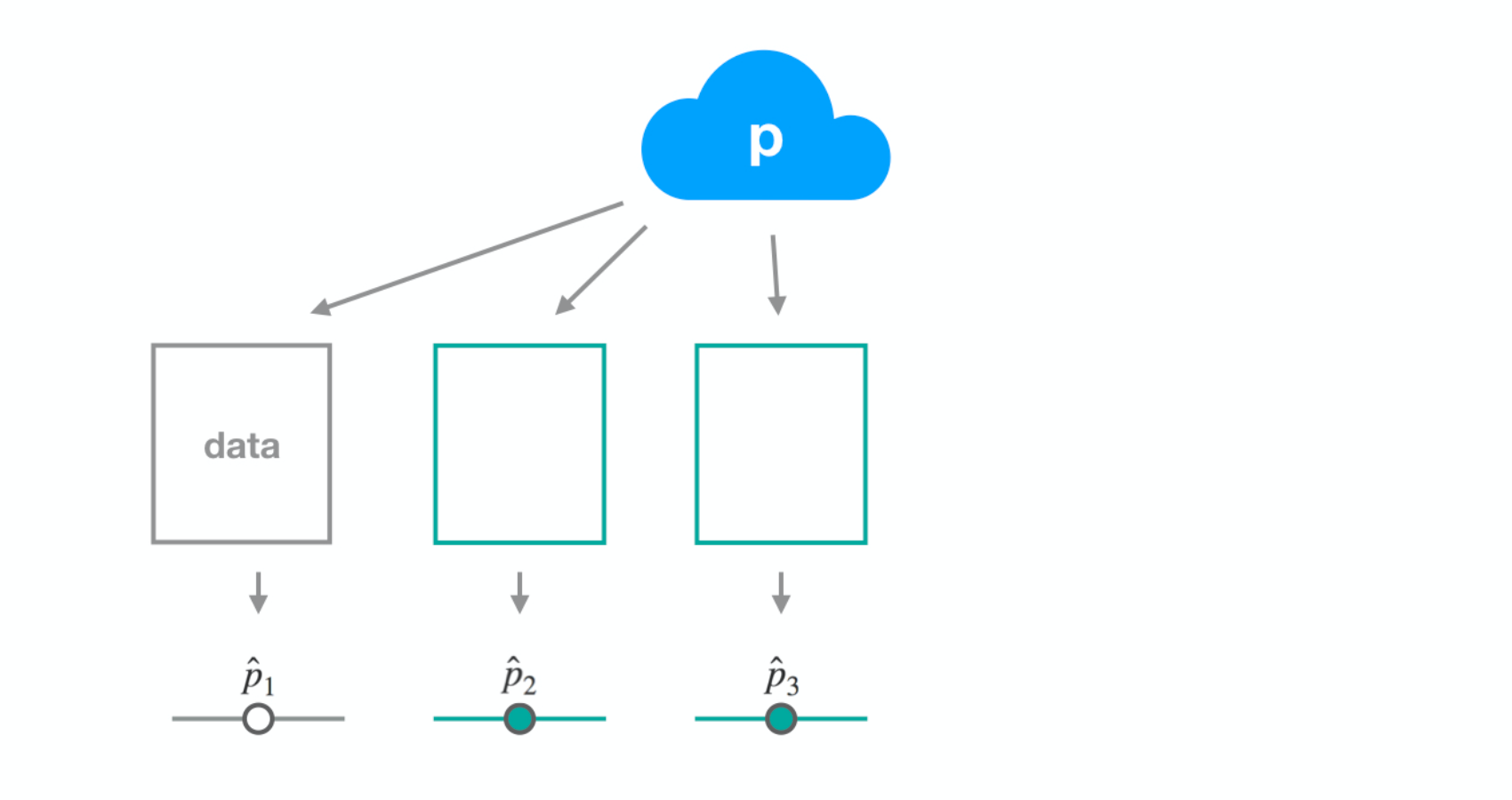
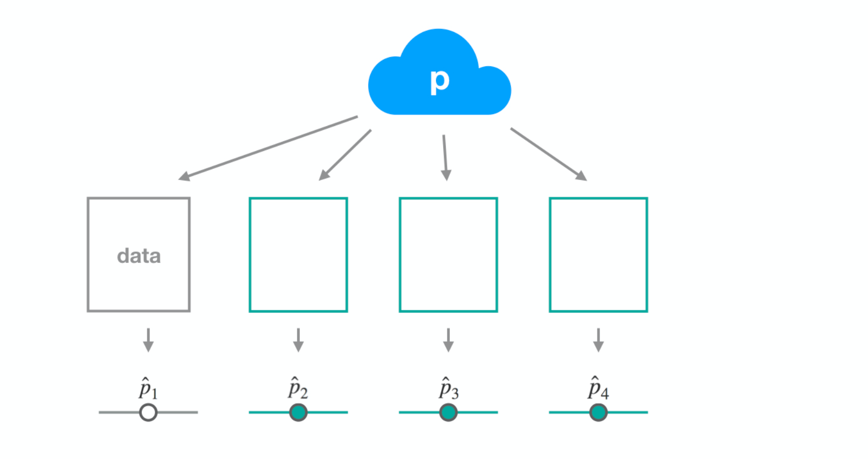
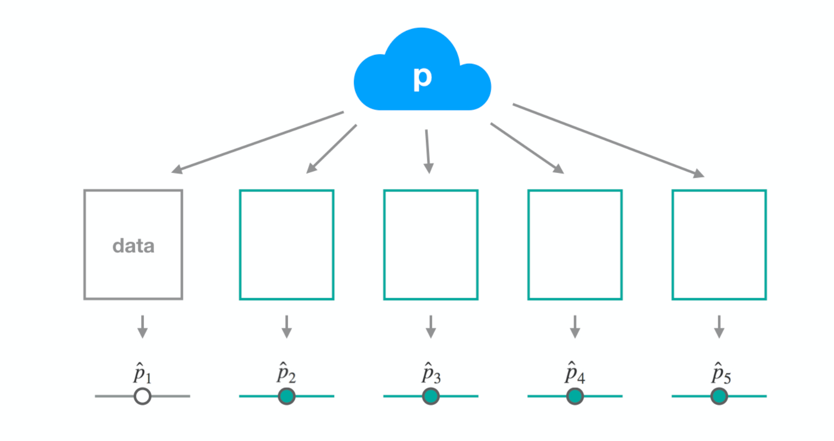
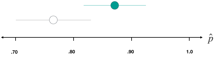
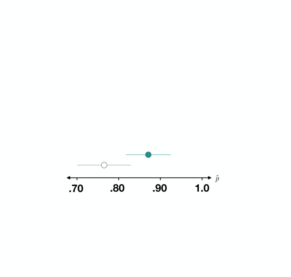
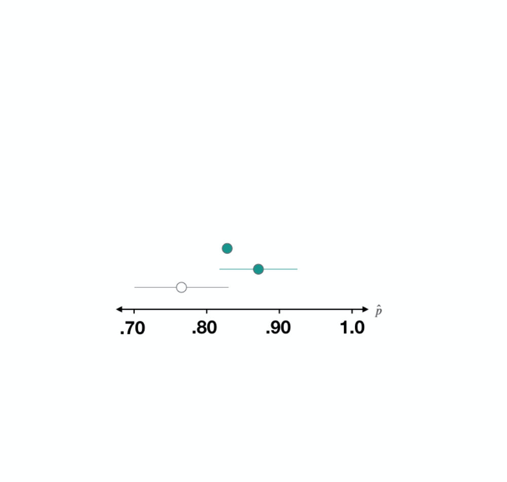
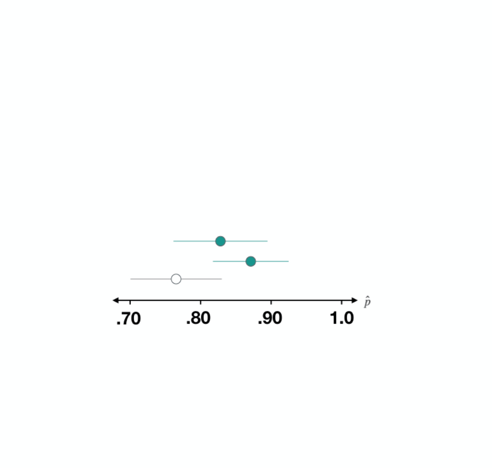
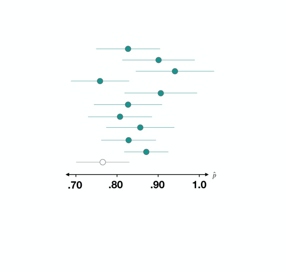
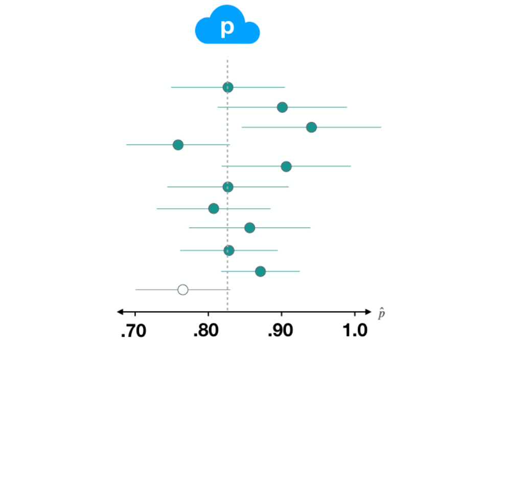
Interpretarea unui interval de încredere

Inferență pentru date categoriale în R

Andrew Bray

Assistant Professor of Statistics at Reed College

Intervale de încredere

Concluzie: proporția reală a americanilor fericiți este între 0,705 și 0,841.

Ce înțelegem prin încredere?

Inferență pentru date categoriale în R

Setul de date 1

ds1 <- filter(gss, year == 2016)

p_hat <- ds1 %>% summarize(mean(happy == "HAPPY")) %>% pull()
SE <- ds1 %>% specify(response = happy, success = "HAPPY") %>% generate(reps = 500, type = "bootstrap") %>% calculate(stat = "prop") %>% summarize(sd(stat)) %>% pull()
c(p_hat - 2 * SE, p_hat + 2 * SE)
0.7073114 0.8393553

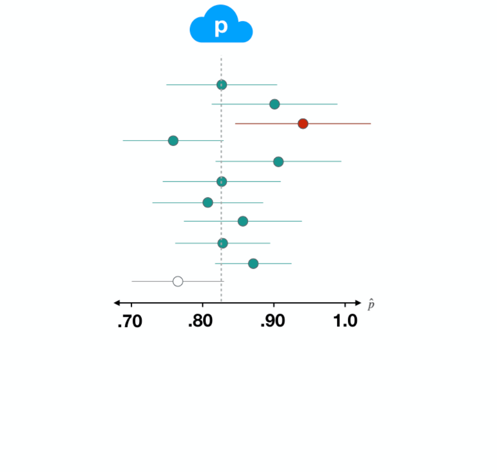
interval de încredere

Inferență pentru date categoriale în R

one.png

Inferență pentru date categoriale în R

two.png

Inferență pentru date categoriale în R

three.png

Inferență pentru date categoriale în R

four.png

Inferență pentru date categoriale în R

five.png

Inferență pentru date categoriale în R

six.png

Inferență pentru date categoriale în R

seven.png

Inferență pentru date categoriale în R

eight.png

Inferență pentru date categoriale în R

nine.png

Inferență pentru date categoriale în R

ten.png

Inferență pentru date categoriale în R

Setul de date 2

ds2 <- filter(gss, year == 2014)

p_hat <- ds1 %>% summarize(mean(happy == "HAPPY")) %>% pull()
SE <- ds1 %>% specify(response = happy, success = "HAPPY") %>% generate(reps = 500, type = "bootstrap") %>% calculate(stat = "prop") %>% summarize(sd(stat)) %>% pull()
c(p_hat - 2 * SE, p_hat + 2 * SE)
0.8348831 0.9384503

Captură de ecran 2019-02-21 18.05.03.png

Inferență pentru date categoriale în R

Setul de date 3

ds3 <- filter(gss, year == 2012)

p_hat <- ds1 %>% summarize(mean(happy == "HAPPY")) %>% pull()
SE <- ds1 %>% specify(response = happy, success = "HAPPY") %>% generate(reps = 500, type = "bootstrap") %>% calculate(stat = "prop") %>% summarize(sd(stat)) %>% pull()
c(p_hat - 2 * SE, p_hat + 2 * SE)
0.7626359 0.8906974

1-2-1.png

Inferență pentru date categoriale în R

Setul de date 3

ds3 <- filter(gss, year == 2012)
p_hat <- ds3 %>%
  summarize(mean(happy == "HAPPY")) %>%
  pull()
SE <- ds3 %>%
  specify(response = happy, 
          success = "HAPPY") %>%
  generate(reps = 500, 
           type = "bootstrap") %>%
  calculate(stat = "prop") %>%
  summarize(sd(stat)) %>%
  pull()

c(p_hat - 2 * SE, p_hat + 2 * SE)
0.7626359 0.8906974

1-2-2.png

Inferență pentru date categoriale în R

Setul de date 3

ds3 <- filter(gss, year == 2012)
p_hat <- ds3 %>%
  summarize(mean(happy == "HAPPY")) %>%
  pull()
SE <- ds3 %>%
  specify(response = happy, 
          success = "HAPPY") %>%
  generate(reps = 500, 
           type = "bootstrap") %>%
  calculate(stat = "prop") %>%
  summarize(sd(stat)) %>%
  pull()

c(p_hat - 2 * SE, p_hat + 2 * SE)
0.7626359 0.8906974

1-2-3.png

Inferență pentru date categoriale în R

Setul de date 3

ds3 <- filter(gss, year == 2012)
p_hat <- ds3 %>%
  summarize(mean(happy == "HAPPY")) %>%
  pull()
SE <- ds3 %>%
  specify(response = happy, 
          success = "HAPPY") %>%
  generate(reps = 500, 
           type = "bootstrap") %>%
  calculate(stat = "prop") %>%
  summarize(sd(stat)) %>%
  pull()

c(p_hat - 2 * SE, p_hat + 2 * SE)
0.7626359 0.8906974

1-2-4.png

Inferență pentru date categoriale în R

Setul de date 3

ds3 <- filter(gss, year == 2012)
p_hat <- ds3 %>%
  summarize(mean(happy == "HAPPY")) %>%
  pull()
SE <- ds3 %>%
  specify(response = happy, 
          success = "HAPPY") %>%
  generate(reps = 500, 
           type = "bootstrap") %>%
  calculate(stat = "prop") %>%
  summarize(sd(stat)) %>%
  pull()

c(p_hat - 2 * SE, p_hat + 2 * SE)
0.7626359 0.8906974

1-2-5.png

Inferență pentru date categoriale în R

Setul de date 3

ds3 <- filter(gss, year == 2012)
p_hat <- ds3 %>%
  summarize(mean(happy == "HAPPY")) %>%
  pull()
SE <- ds3 %>%
  specify(response = happy, 
          success = "HAPPY") %>%
  generate(reps = 500, 
           type = "bootstrap") %>%
  calculate(stat = "prop") %>%
  summarize(sd(stat)) %>%
  pull()

c(p_hat - 2 * SE, p_hat + 2 * SE)
0.7626359 0.8906974

1-2-6.png

Inferență pentru date categoriale în R

Intervale de încredere

Interpretare: „Suntem 95% siguri că proporția reală a americanilor fericiți este între 0,705 și 0,841."

Lățimea intervalului este influențată de

  • n
  • nivelul de încredere
  • p
Inferență pentru date categoriale în R

Să exersăm!

Inferență pentru date categoriale în R

Preparing Video For Download...