Faceting plotly graphics

Interactive Data Visualization with plotly in R

Adam Loy

Statistician, Carleton College

2016 video game sales

glimpse(vgsales2016)

Rows: 502
Columns: 16
$ Name         <fct> FIFA 17, Pokemon Sun/Moon, Unchart...
$ Platform     <fct> PS4, 3DS, PS4, PS4, PS4, PS4, XOne...
$ Year         <int> 2016, 2016, 2016, 2016, 2016, 2016...
$ Genre        <fct> Sports, Role-Playing, Shooter, Sho...
$ Publisher    <fct> Electronic Arts, Nintendo, Sony Co...
$ NA_Sales     <dbl> 0.66, 2.98, 1.85, 1.61, 1.10, 1.35...
...
$ User_Score   <fct> 5, NA, 7.9, 3.4, 8.4, 7, 5.5, 3.1,...
$ User_Count   <int> 398, NA, 7064, 1129, 809, 2219, 20...
$ Developer    <fct> EA Sports, EA Vancouver, NA, Naugh...
$ Rating       <fct> E, NA, T, M, M, M, E, M, M, M, M, ...

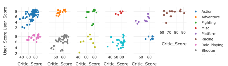
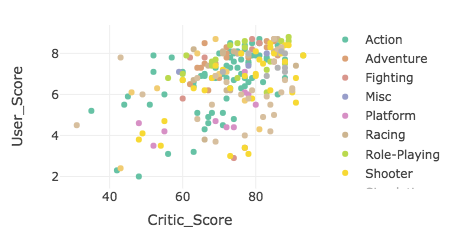
Representing many categories

vgsales2016 %>%
  plot_ly(x = ~Critic_Score, y = ~User_Score, color = ~Genre) %>%
  add_markers()

A single subplot

library(dplyr)
action_df <- vgsales2016 %>%
  filter(Genre == "Action")

glimpse(action_df)

Rows: 178
Columns: 16
$ Name         <fct> Far Cry: Primal, Mafia III, No Man's Sky, Yokai Watch 3, Watch Do...
$ Platform     <fct> PS4, PS4, PS4, 3DS, PS4, WiiU, 3DS, PS4, XOne, PS4, PS4, PS4, PS4...
$ Year         <int> 2016, 2016, 2016, 2016, 2016, 2016, 2016, 2016, 2016, 2016, 2016,...
$ Genre        <fct> Action, Action, Action, Action, Action, Action, Action, Action, A...
$ Publisher    <fct> Ubisoft, Take-Two Interactive, Hello Games, Level 5, Ubisoft, Nin...
$ NA_Sales     <dbl> 0.60, 0.42, 0.63, 0.00, 0.37, 0.56, 0.28, 0.72, 0.47, 0.26, 0.24,...
...

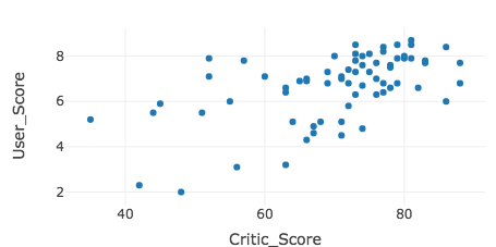
A single subplot

action_df %>%
  plot_ly(x = ~Critic_Score, y = ~User_Score) %>%
  add_markers()

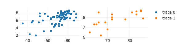
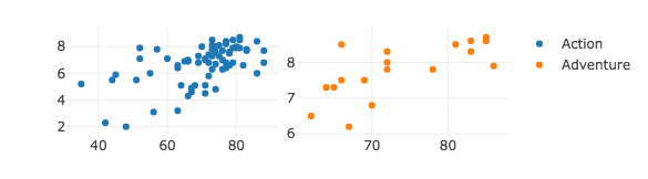
Two subplots

p1 <- action_df %>%
  plot_ly(x = ~Critic_Score, y = ~User_Score) %>%
  add_markers()

p2 <- vgsales2016 %>%
  filter(Genre == "Adventure") %>%
  plot_ly(x = ~Critic_Score, y = ~User_Score) %>%
  add_markers()

subplot(p1, p2, nrows = 1)

Legends

p1 <- plot_ly(x = ~Critic_Score, y = ~User_Score) %>%
  add_markers(name = ~Genre) 

p2 <- vgsales2016 %>%
  filter(Genre == "Adventure") %>%
  plot_ly(x = ~Critic_Score, y = ~User_Score) %>%
  add_markers(name = ~Genre) 

subplot(p1, p2, nrows = 1)

Axis labels

subplot(p1, p2, nrows = 1, shareY = TRUE, shareX = TRUE)

Sharing an axis leads to linked interactivity
If linked interactivity is not desired: use titleX and titleY arguments

Iterate to automate

library(tidyverse)

vgsales2016 %>%
  group_by(Genre) %>%
  nest()

# A tibble: 12 × 2
# Groups:   Genre [12]
   Genre        data               
   <chr>        <list>             
 1 Sports       <tibble [48 × 15]> 
 2 Role-Playing <tibble [54 × 15]> 
 3 Shooter      <tibble [47 × 15]> 
 4 Action       <tibble [178 × 15]>
 5 Platform     <tibble [15 × 15]> 
 6 Fighting     <tibble [16 × 15]> 
 7 Racing       <tibble [24 × 15]> 
 8 Adventure    <tibble [56 × 15]> 
 9 Misc         <tibble [32 × 15]> 
10 Simulation   <tibble [18 × 15]> 
11 Strategy     <tibble [13 × 15]> 
12 Puzzle       <tibble [1 × 15]>

Iterate to automate

library(tidyverse)
vgsales2016 %>%
  group_by(Genre) %>%
  nest() %>%

  mutate(
    plot = map2(data, Genre,
      \(data, Genre) 
      plot_ly(data = data, 
          x = ~Critic_Score, 
          y = ~User_Score) %>%
      add_markers(name = ~Genre)
    ))

# A tibble: 12 × 3
# Groups:   Genre [12]
   Genre        data                plot    
   <chr>        <list>              <list>  
 1 Sports       <tibble [48 × 15]>  <plotly>
 2 Role-Playing <tibble [54 × 15]>  <plotly>
 3 Shooter      <tibble [47 × 15]>  <plotly>
 4 Action       <tibble [178 × 15]> <plotly>
 5 Platform     <tibble [15 × 15]>  <plotly>
 6 Fighting     <tibble [16 × 15]>  <plotly>
 7 Racing       <tibble [24 × 15]>  <plotly>
 8 Adventure    <tibble [56 × 15]>  <plotly>
 9 Misc         <tibble [32 × 15]>  <plotly>
10 Simulation   <tibble [18 × 15]>  <plotly>
11 Strategy     <tibble [13 × 15]>  <plotly>
12 Puzzle       <tibble [1 × 15]>   <plotly>

Iterate to automate

vgsales2016 %>%
  group_by(Genre) %>%
  nest() %>%
  mutate(
    plot = map2(
      data, Genre,
      \(data, Genre) 
       plot_ly(data = data, 
          x = ~Critic_Score, 
          y = ~User_Score) %>%
      add_markers(name = ~Genre)
    )) %>%

  subplot(nrows = 2)

Let's practice!

Interactive Data Visualization with plotly in R