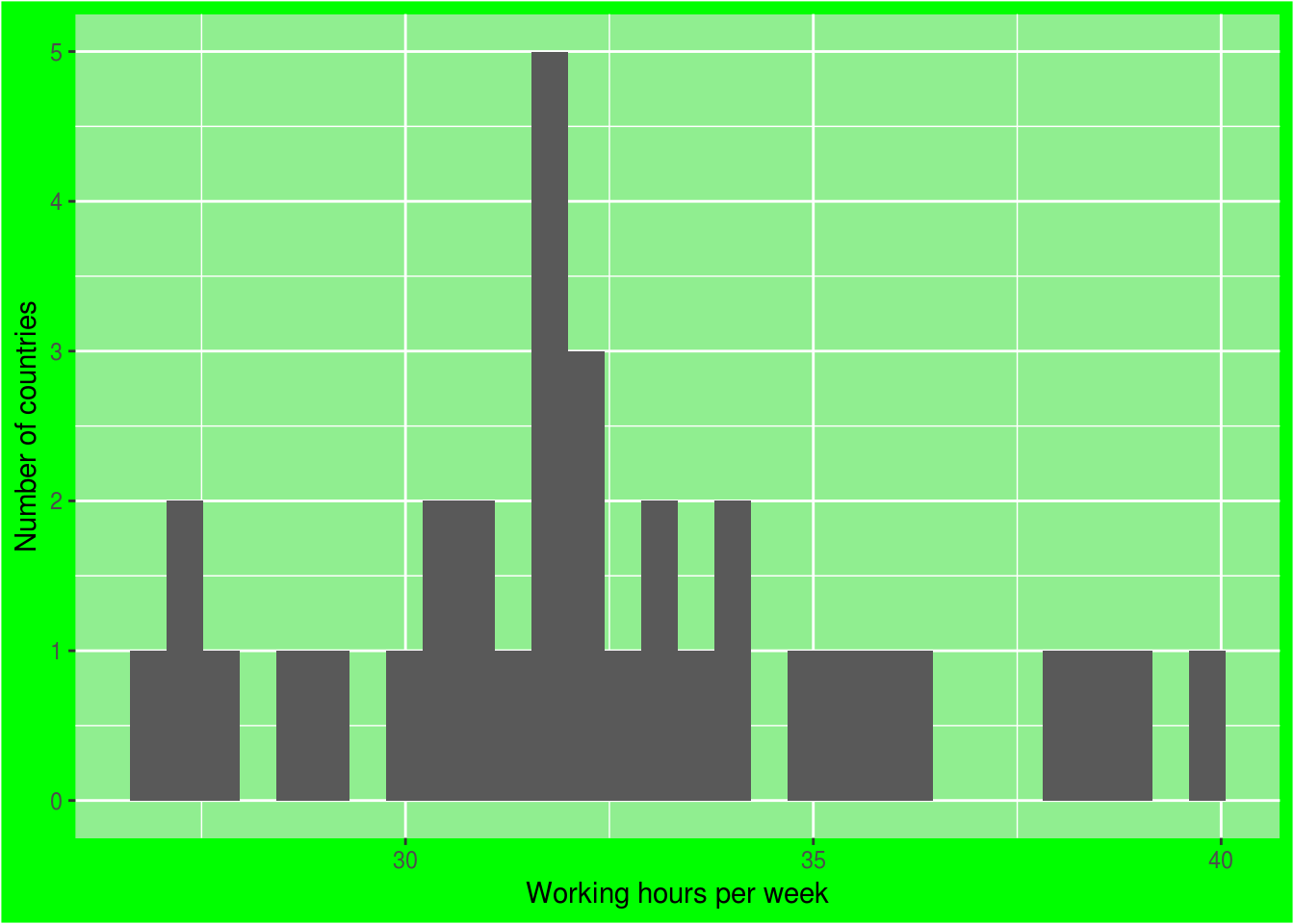
Visualizing aspects of data with facets

Communicating with Data in the Tidyverse

Timo Grossenbacher

Data Journalist

The facet_grid() function

ilo_data <- ilo_data %>%
  filter(year == "1996" | year == "2006") 
ilo_plot <- ggplot(ilo_data) +
  geom_histogram(aes(
    x = working_hours)) +
  labs(x = "Working hours per week",
       y = "Number of countries")

ilo_plot +
  facet_grid(cols = vars(year))

ilo_plot +
  facet_grid(rows = vars(year))

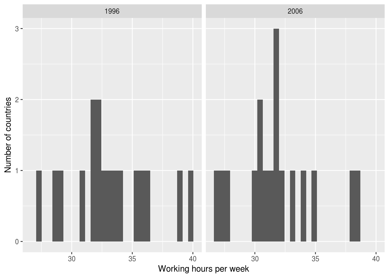
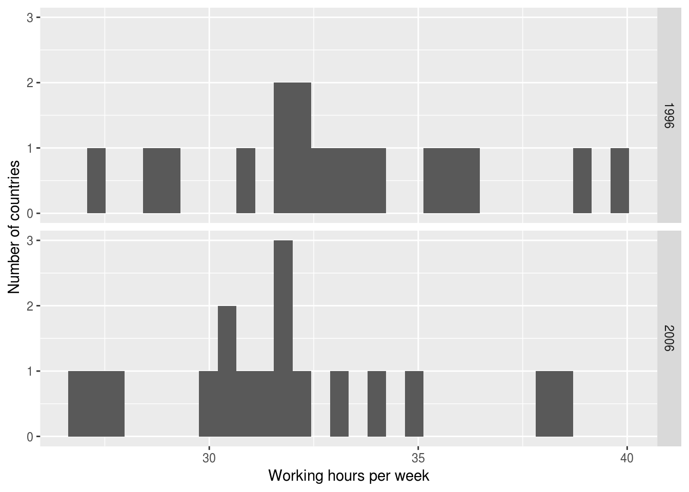
The facet_grid() function

ilo_data <- ilo_data %>%
  filter(year == "1996" | year == "2006")
ggplot(ilo_data) +
  geom_histogram(aes(x = working_hours)) +
  labs(x = "Working hours per week",
       y = "Number of countries") +
  facet_grid(cols = vars(year))

ggplot(ilo_data) +
  geom_histogram(aes(x = working_hours)) +
  labs(x = "Working hours per week",
       y = "Number of countries") +
  facet_wrap(facets = vars(year))

A faceted scatter plot

Styling faceted plots

strip.background
strip.text
...

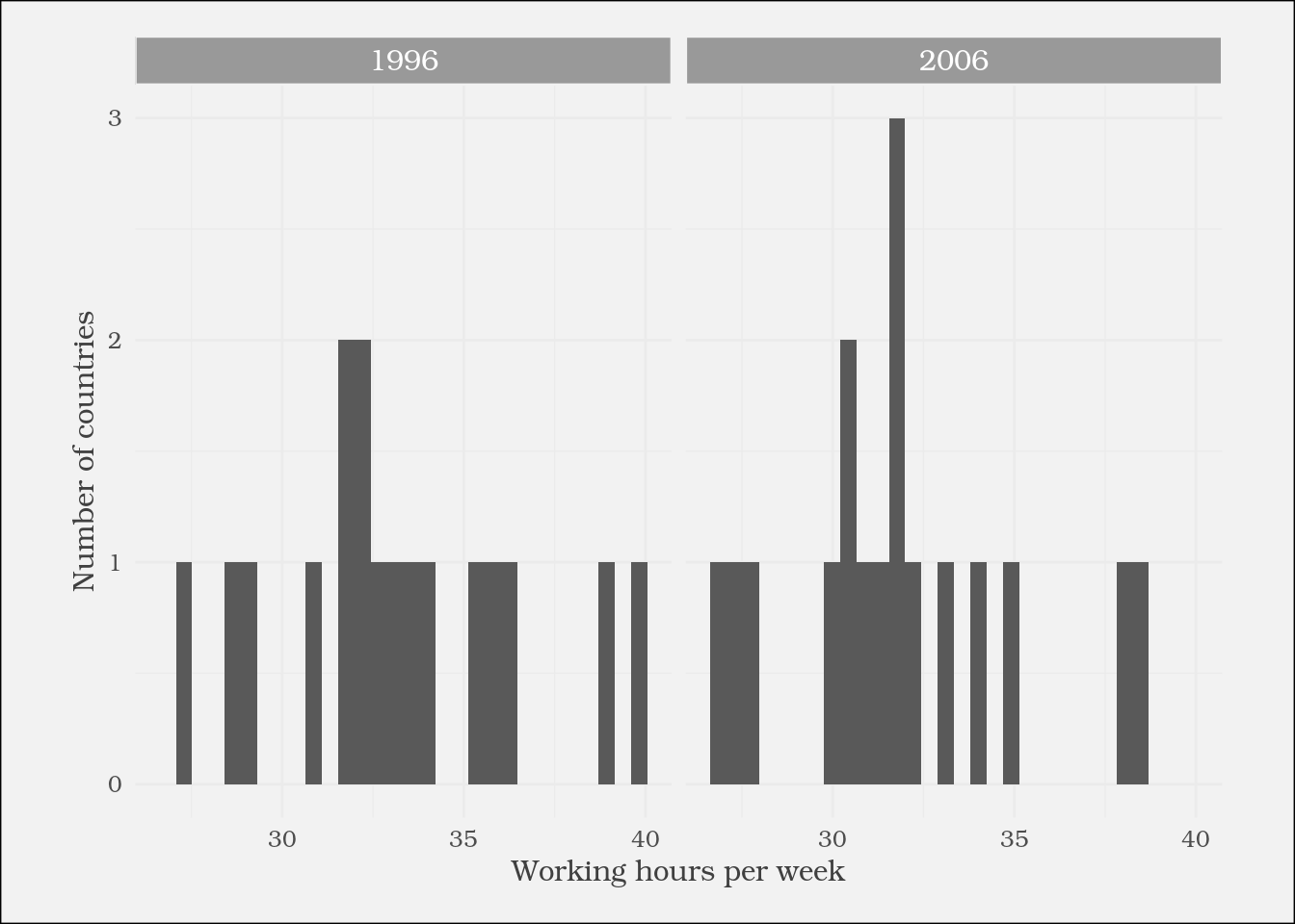
Defining your own theme function

theme_green <- function(){
  theme(
    plot.background = 
      element_rect(fill = "green"),
    panel.background = 
      element_rect(fill = 
        "lightgreen")
  )}

ggplot(ilo_data) +
  geom_histogram(aes(
    x = working_hours)) +
  labs(x = "Working hours per week",
       y = "Number of countries") +

theme_green()

Let's practice!

Communicating with Data in the Tidyverse