Filtering and plotting the data

Communicating with Data in the Tidyverse

Timo Grossenbacher

Data Journalist

Filter the data for European countries

ilo_data %>%
  filter(country == "Switzerland")

# A tibble: 27 x 4
       country   year hourly_compensation working_hours
         <fct>  <fct>               <dbl>         <dbl>
 1 Switzerland   1980               10.96      34.70385
 2 Switzerland   1981               10.01      34.33462
 3 Switzerland   1982               10.31      34.12308
 4 Switzerland   1983               10.33      33.84231
 5 Switzerland   1984                9.52      33.47885
 6 Switzerland   1985                9.55      33.35961
 7 Switzerland   1986               13.62      33.19615
 8 Switzerland   1987               16.90      33.17308
 9 Switzerland   1988               17.81      33.16269
10 Switzerland   1989               16.54      32.87308
# ... with 17 more rows

ilo_data %>% 
  filter(country %in% c("Sweden", "Switzerland"))

# A tibble: 54 x 4
      country   year hourly_compensation working_hours
        <fct>  <fct>               <dbl>         <dbl>
1      Sweden   1980               12.40      29.16923
2 Switzerland   1980               10.96      34.70385
3      Sweden   1981               11.70      29.00769
4 Switzerland   1981               10.01      34.33462
5      Sweden   1982                9.99      29.27885
# ... with 49 more rows

...equivalent to:

ilo_data %>% 
  filter(country == "Sweden" | country == "Switzerland")

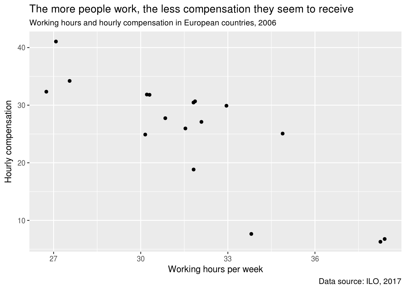
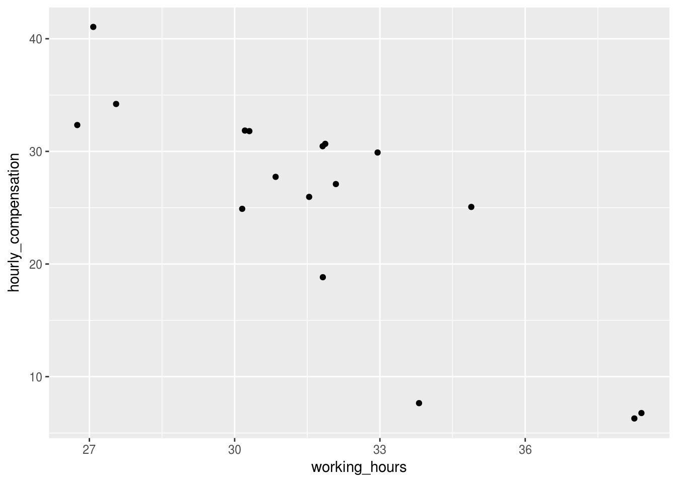
The relationship between both indicators

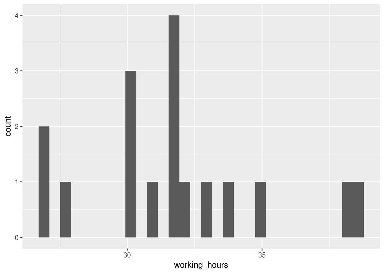
plot_data <- 
  ilo_data %>% 
    filter(year == 2006)

ggplot(plot_data) +
  geom_histogram(
    aes(x = working_hours))

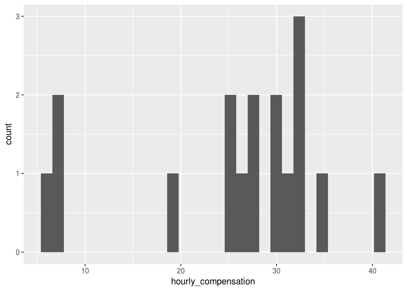
plot_data <- 
  ilo_data %>% 
    filter(year == 2006)

ggplot(plot_data) +
  geom_histogram(
    aes(x = hourly_compensation))

The relationship between both indicators

Adding labels to the plot

Some dplyr function repetition

ilo_data %>%
  group_by(country) %>% 
  summarize(median_working_hours = median(working_hours))

# A tibble: 17 x 2
     country median_working_hours
       <fct>                <dbl>
1    Austria             31.69904
2    Belgium             32.03846
3 Czech Rep.             39.10000
4    Finland             34.04808
5     France             32.34615
# ... with 12 more rows

Let's practice!

Communicating with Data in the Tidyverse