Introduction au bootstrap

Échantillonnage en R

Richie Cotton

Data Evangelist at DataCamp

Avec ou sans

Échantillonnage sans remise

Cartes à jouer sur une table de casino.

Échantillonnage avec remise (« rééchantillonnage »)

Quatre dés qui roulent.

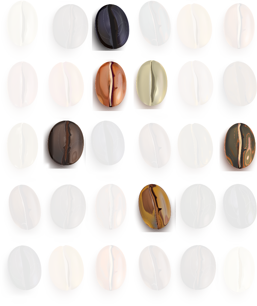
Échantillonnage aléatoire simple sans remise

Population

Grains de café disposés en rangées et colonnes.

Échantillon

Grains de café en rangées et colonnes, dont la plupart sont grisés.

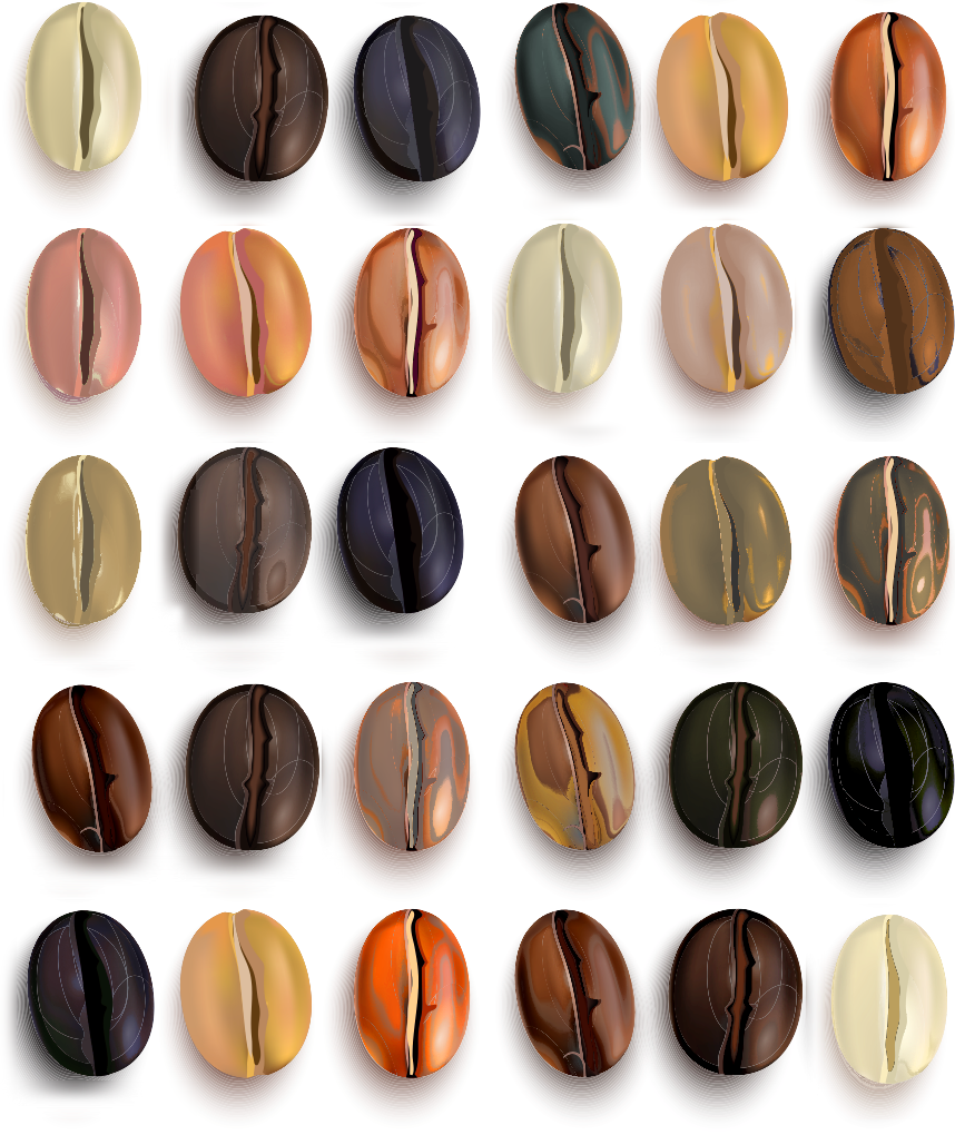
Échantillonnage aléatoire simple avec remise

Population

Grains de café disposés en rangées et colonnes.

Échantillon

Un échantillon aléatoire de grains de café, dont certains en double.

Pourquoi échantillonner avec remise ?

Considérez les données coffee_ratings comme un échantillon d'une plus grande population de cafés.
Considérez chaque café de l'échantillon comme représentant plusieurs cafés absents de l'échantillon mais présents dans la population.
L'échantillonnage avec remise sert de substitut pour inclure différents membres de ces groupes dans l'échantillon.

Préparer les données sur le café

coffee_focus <- coffee_ratings %>%
  select(variety, country_of_origin, flavor) %>%
  rowid_to_column()

glimpse(coffee_focus)

Rows: 1,338
Columns: 4
$ rowid             <int> 1, 2, 3, 4, 5, 6, 7, 8, 9, 10, 11, 12, 13, 14, 15, ...
$ variety           <chr> NA, "Other", "Bourbon", NA, "Other", NA, "Other", N...
$ country_of_origin <chr> "Ethiopia", "Ethiopia", "Guatemala", "Ethiopia", "E...
$ flavor            <dbl> 8.83, 8.67, 8.50, 8.58, 8.50, 8.42, 8.50, 8.33, 8.6...

Rééchantillonner avec slice_sample()

coffee_resamp <- coffee_focus %>%
  slice_sample(prop = 1, replace = TRUE)

# A tibble: 1,338 x 4
   rowid variety country_of_origin flavor
   <int> <chr>   <chr>              <dbl>
 1  1253 Bourbon Guatemala           6.92
 2   186 Caturra Colombia            7.58
 3  1185 Bourbon Guatemala           7.42
 4  1273 NA      Philippines         6.5 
 5  1042 Caturra Honduras            7.33
 6   195 Caturra Guatemala           7.75
 7  1219 Typica  Mexico              7   
 8   952 Caturra Honduras            7.5 
 9    41 Caturra Thailand            8.33
10   460 Caturra Honduras            7.67
# ... with 1,328 more rows

Cafés répétés

coffee_resamp %>% 
  count(rowid, sort = TRUE)

# A tibble: 844 x 2
   rowid     n
   <int> <int>
 1   704     5
 2   913     5
 3  1070     5
 4    16     4
 5   180     4
 6   230     4
 7   234     4
 8   342     4
 9   354     4
10   423     4
# ... with 834 more rows

Cafés manquants

coffee_resamp %>% 
  summarize(
    coffees_included = n_distinct(rowid),
    coffees_not_included = n() - coffees_included
  )

# A tibble: 1 x 2
  coffees_included coffees_not_included
             <int>                <int>
1              844                  494

Bootstrap

L'inverse de l'échantillonnage à partir d'une population.

Échantillonnage : passer d'une population à un plus petit échantillon.

Bootstrap : construire une population théorique à partir de votre échantillon.

Cas d'usage du bootstrap

Comprendre la variabilité d'échantillonnage à partir d'un seul échantillon.

Une botte de cowboy.

Processus de bootstrap

Créer un rééchantillon de même taille que l'échantillon initial.
Calculer la statistique d'intérêt pour cet échantillon bootstrap.
Répéter les étapes 1 et 2 plusieurs fois.

Les statistiques obtenues sont des statistiques bootstrap et, lorsqu'on les examine pour leur variabilité, forment une distribution bootstrap.

Bootstrap de la saveur moyenne du café

# Step 3. Repeat many times
mean_flavors_1000 <- replicate(
  n = 1000,
  expr = {

    coffee_focus %>%
      # Step 1. Resample
      slice_sample(prop = 1, replace = TRUE) %>%

      # Step 2. Calculate statistic
      summarize(mean_flavor = mean(flavor, na.rm = TRUE)) %>% 
      pull(mean_flavor)

})

Histogramme de la distribution bootstrap

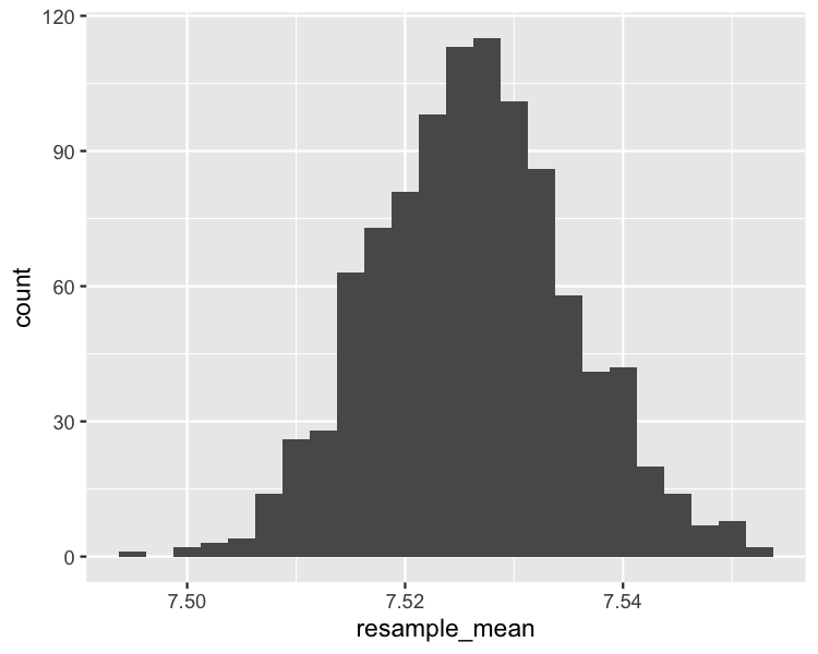
bootstrap_distn <- tibble(
  resample_mean = mean_flavors_1000
)

ggplot(bootstrap_distn, aes(resample_mean)) +
  geom_histogram(binwidth = 0.0025)

Histogramme de la distribution bootstrap de la moyenne d'échantillon.

Passons à la pratique !

Échantillonnage en R