Comparer les distributions d'échantillonnage et de bootstrap

Échantillonnage en R

Richie Cotton

Data Evangelist at DataCamp

Sous-ensemble axé sur le café

set.seed(19790801)
coffee_sample <- coffee_ratings %>%
  select(variety, country_of_origin, flavor) %>%
  rowid_to_column() %>% 
  slice_sample(n = 500)
glimpse(coffee_sample)

Rows: 500
Columns: 4
$ rowid             <int> 10, 278, 458, 622, 131, 385, 1292, 47, 904, 1020, 5...
$ variety           <chr> "Other", "Bourbon", NA, "Caturra", "Caturra", "Yell...
$ country_of_origin <chr> "Ethiopia", "Guatemala", "Colombia", "Thailand", "C...
$ flavor            <dbl> 8.58, 7.75, 7.75, 7.50, 8.00, 7.83, 7.17, 8.08, 7.3...

Bootstrap de la moyenne des saveurs de café

mean_flavors_1000 <- replicate(
  n = 1000,
  expr = coffee_sample %>%
    slice_sample(prop = 1, replace = TRUE) %>%
    summarize(mean_flavor = mean(flavor, na.rm = TRUE)) %>%
    pull(mean_flavor)
)
bootstrap_distn <- tibble(
  resample_mean = mean_flavors_1000
)

Distribution bootstrap de la moyenne des saveurs

 ggplot(bootstrap_distn, aes(resample_mean)) +
  geom_histogram(binwidth = 0.0025)

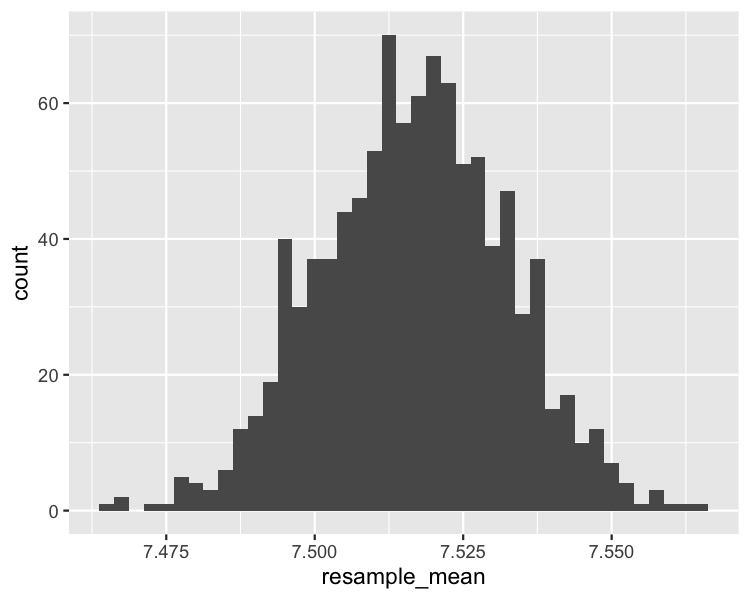
Histogramme de la distribution bootstrap.

Moyennes : échantillon, distribution bootstrap, population

Moyenne de l'échantillon

coffee_sample %>% 
  summarize(mean_flavor = mean(flavor)) %>% 
  pull(mean_flavor)

7.5163

Moyenne de la population estimée

bootstrap_distn %>% 
  summarize(mean_mean_flavor = mean(resample_mean)) %>% 
  pull(mean_mean_flavor)

7.5167

Vraie moyenne de la population

coffee_ratings %>% 
  summarize(mean_flavor = mean(flavor)) %>% 
  pull(mean_flavor)

7.5260

Interpréter les moyennes

La moyenne de la distribution bootstrap est presque identique à la moyenne d'échantillon.
Elle peut mal estimer la moyenne de la population.
Le bootstrap ne corrige pas les biais dus aux écarts entre votre échantillon et la population.

Écart-type : échantillon vs distribution bootstrap

Écart-type de l'échantillon

coffee_focus %>% 
  summarize(sd_flavor = sd(flavor)) %>% 
  pull(sd_flavor)

0.3525

Écart-type de la population estimé ?

bootstrap_distn %>% 
  summarize(sd_mean_flavor = sd(resample_mean)) %>% 
  pull(sd_mean_flavor)

0.01572

Écarts-types : échantillon, dist. bootstrap, population

Écart-type de l'échantillon

coffee_focus %>% 
  summarize(sd_flavor = sd(flavor)) %>% 
  pull(sd_flavor)

0.3525

Écart-type de la population estimé

standard_error <- bootstrap_distn %>%
  summarize(sd_mean_flavor = sd(resample_mean)) %>% 
  pull(sd_mean_flavor)

standard_error * sqrt(500)

0.3515

Vrai écart-type

coffee_ratings %>%
  summarize(sd_flavor = sd(flavor)) %>%
  pull(sd_flavor)

0.3414

L'« erreur-type » est l'écart-type de la statistique d'intérêt.

L'« erreur-type » multipliée par la racine carrée de la taille de l'échantillon estime l'écart-type populationnel.

Interpréter les erreurs-types

L'« erreur-type estimée » est l'écart-type de la distribution bootstrap d'une statistique d'échantillon.
L'« erreur-type de la distribution bootstrap » multipliée par la racine carrée de la taille d'échantillon estime l'écart-type dans la population.

Passons à la pratique !

Échantillonnage en R