Échantillonnage de commodité

Échantillonnage en R

Richie Cotton

Data Evangelist at DataCamp

La prédiction du Literary Digest

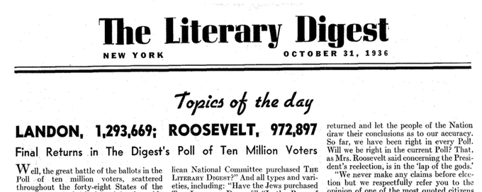
La une du Literary Digest de 1936 annonçant des prédictions électorales. On prévoyait 1,3 million de votes pour Landon et un peu moins d'un million pour Roosevelt.

Prédiction : Landon 57 %; Roosevelt 43 %
Résultats réels : Landon 38 %; Roosevelt 62 %
Échantillon non représentatif de la population : biais d'échantillonnage.
Recueillir des données par la méthode la plus facile = échantillonnage de commodité.

Trouver l'âge moyen des Français

Une photo de Disneyland Paris.

Sonder 10 personnes à Disneyland Paris.
Leur âge moyen est de 24,6 ans.
Est-ce une bonne estimation pour toute la France ?

¹ Image par Sean MacEntee

Quelle était la précision du sondage ?

Année	Âge moyen en France
1975	31,6
1985	33,6
1995	36,2
2005	38,9
2015	41,2

24,6 ans est une piètre estimation.
Les visiteurs de Disneyland ne représentent pas l'ensemble de la population.

Échantillonnage de commodité : cotes de café

coffee_ratings %>% 
  summarize(mean_cup_points = mean(total_cup_points))

  mean_cup_points
1           82.09

coffee_ratings_first10 <- coffee_ratings %>% 
  slice_head(n = 10)

coffee_ratings_first10 %>% 
  summarize(mean_cup_points = mean(total_cup_points))

  mean_cup_points
1            89.1

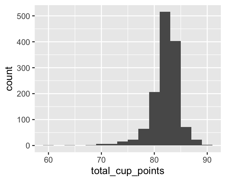
Visualiser le biais de sélection

coffee_ratings %>%
  ggplot(aes(x = total_cup_points)) +
  geom_histogram(binwidth = 2)

Un histogramme des points de tasse pour la population.

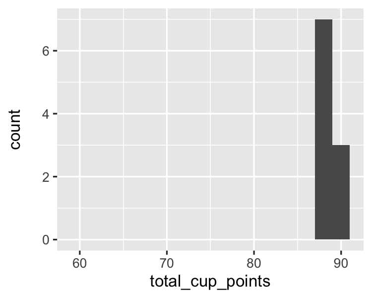
coffee_ratings_first10 %>%
  ggplot(aes(x = total_cup_points)) +
  geom_histogram(binwidth = 2) +
  xlim(59, 91)

Un histogramme des points de tasse pour l'échantillon.

Visualiser le biais de sélection 2

coffee_ratings %>%
  ggplot(aes(x = total_cup_points)) +
  geom_histogram(binwidth = 2)

Un histogramme des points de tasse pour la population.

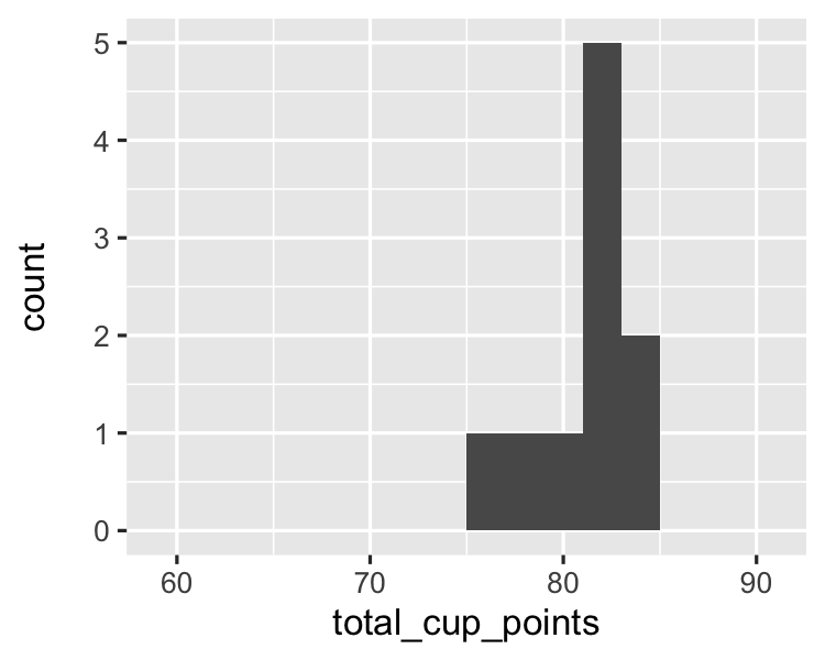
coffee_ratings %>%
  slice_sample(n = 10) %>% 
  ggplot(aes(x = total_cup_points)) +
  geom_histogram(binwidth = 2) +
  xlim(59, 91)

Un histogramme des points de tasse pour un échantillon aléatoire.

Passons à la pratique !

Échantillonnage en R