Formulation d'hypothèses et distributions

A/B Testing en Python

Moe Lotfy, PhD

Principal Data Science Manager

Définir des hypothèses

Une hypothèse, c'est :
- une proposition qui explique un événement
- un point de départ pour approfondir l'analyse
- une idée à mettre à l'épreuve
Une bonne hypothèse :
- est vérifiable, déclarative, concise et logique
- permet une itération systématique
- se généralise plus facilement et clarifie la compréhension
- mène à des recommandations concrètes et ciblées

Format d'hypothèse

Gabarit général :
- Selon X, nous croyons que si nous faisons Y
- Alors Z se produira
- Tel que mesuré par la(les) mesure(s) M
Exemple d'hypothèse alternative :
- D'après la recherche sur l'expérience utilisateur, nous croyons que si nous mettons à jour la conception de la page de paiement
- Alors le pourcentage de clients achetant augmentera
- Tel que mesuré par le taux d'achat
Hypothèse nulle : …le pourcentage de clients achetant ne changera pas…

Calculer des statistiques d'échantillon

# Calculate the number of users in groups A and B
n_A = checkout[checkout['checkout_page'] == 'A']['purchased'].count()
n_B = checkout[checkout['checkout_page'] == 'B']['purchased'].count()
print('Group A users:',n_A)
print('Group B users:',n_B)

Group A users: 3000
Group B users: 3000

# Calculate the mean purchase rates of groups A and B
p_A = checkout[checkout['checkout_page'] == 'A']['purchased'].mean()
p_B = checkout[checkout['checkout_page'] == 'B']['purchased'].mean()
print('Group A mean purchase rate:',p_A)
print('Group B mean purchase rate:',p_B)

Group A mean purchase rate: 0.820
Group B mean purchase rate: 0.847

Simuler et tracer des distributions

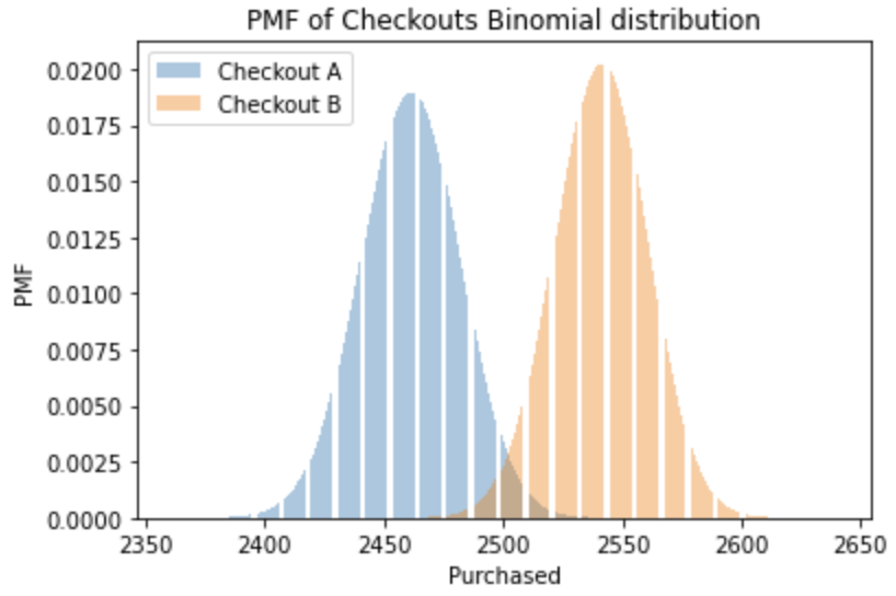
Le nombre d'acheteurs sur n essais, avec une probabilité d'achat p, suit une loi binomiale.

# Import binom from scipy library 
from scipy.stats import binom 
# Create x-axis range and Binomial distributions A and B
x = np.arange(n_A*p_A - 100, n_B*p_B + 100) 
binom_a = binom.pmf(x, n_A, p_A)
binom_b = binom.pmf(x, n_B, p_B) 
# Plot Binomial distributions A and B
plt.bar(x, binom_a, alpha=0.4, label='Checkout A')
plt.bar(x, binom_b, alpha=0.4, label='Checkout B')
plt.xlabel('Purchased')
plt.ylabel('PMF')
plt.title('PMF of Checkouts Binomial distribution')
plt.show()

Distribution binomiale des groupes de passage à la caisse A et B

Théorème central limite

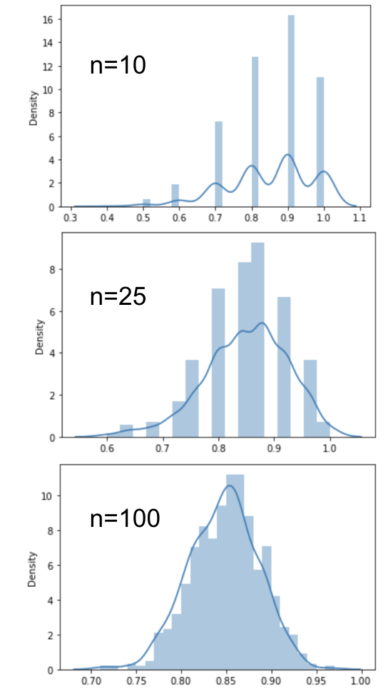
Pour un échantillon assez grand, la distribution des moyennes d'échantillon, p, sera

normale autour de la vraie moyenne de la population
avec un écart-type = erreur-type de la moyenne
quelle que soit la distribution des données sous-jacentes

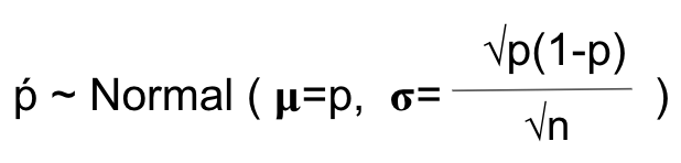
Formule du théorème central limite pour des proportions

Théorème central limite en Python

# Set random seed for repeatability 
np.random.seed(47)
# Create an empty list to hold means
sampled_means = []
# Create loop to simulate 1000 sample means
for i in range(1000):
    # Take a sample of n=100
    sample = checkout['purchased'].sample(100,replace=True)
    # Get the sample mean and append to list
    sample_mean = np.mean(sample)
    sampled_means.append(sample_mean)
# Plot distribution
sns.displot(sampled_means, kde=True)
plt.show()

Démonstration en Python du théorème central limite. La distribution tend vers une loi normale à mesure que la taille de l'échantillon augmente

Représentation mathématique d'une hypothèse

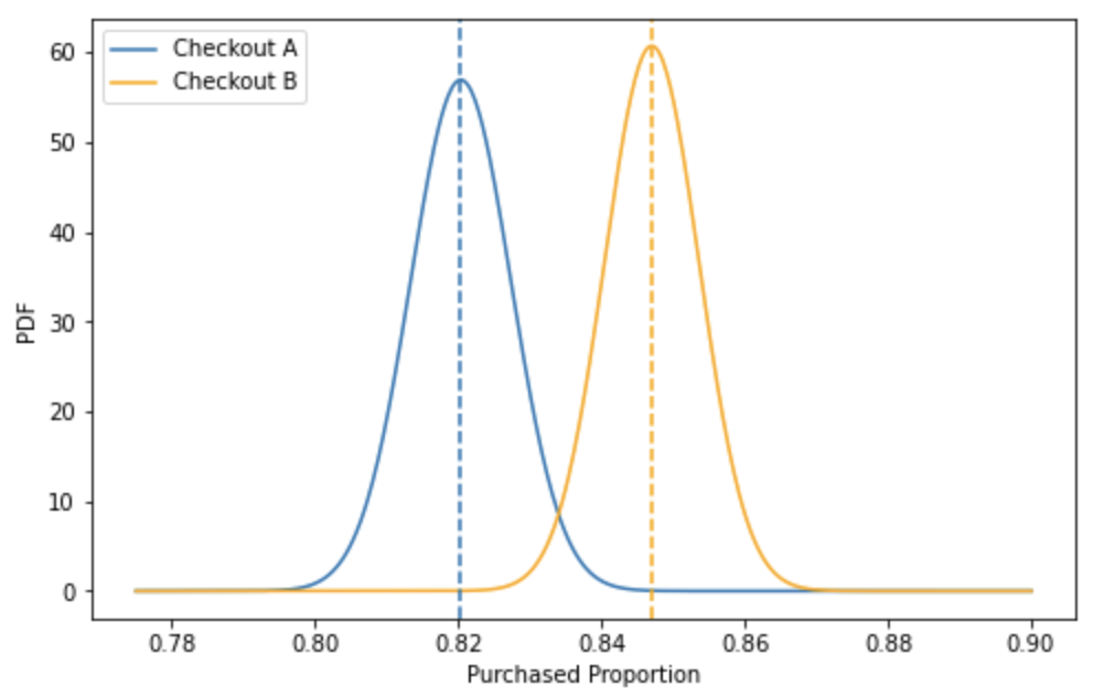
# Import norm from scipy library 
from scipy.stats import norm
# Create x-axis range and normal distributions A and B
x = np.linspace(0.775, 0.9, 500)
norm_a = norm.pdf(x, p_A, np.sqrt(p_A*(1-p_A) / n_A))
norm_b = norm.pdf(x, p_B, np.sqrt(p_B*(1-p_B) / n_B))
# Plot normal distributions A and B
sns.lineplot(x=x, y=norm_a, ax=ax, label='Checkout A')
sns.lineplot(x=x, y=norm_b, color='orange', \
             ax=ax, label= 'Checkout B')
ax.axvline(p_A, linestyle='--')
ax.axvline(p_B, linestyle='--')
plt.xlabel('Purchased Proportion')
plt.ylabel('PDF')
plt.legend(loc="upper left")
plt.show()

Graphiques de différence de moyennes pour les hypothèses nulle et alternative

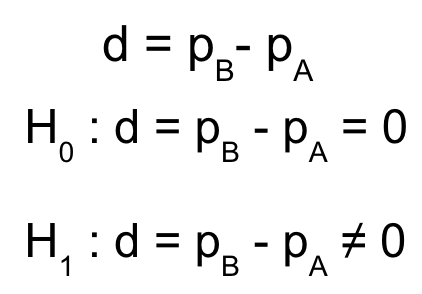
Formulation mathématique des hypothèses nulle et alternative

Passons à la pratique !

A/B Testing en Python