Introduction à l'analyse de portefeuille en Python
Charlotte Werger
Data Scientist
$$
$$


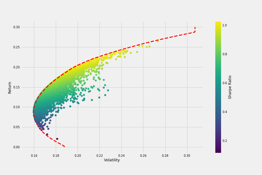
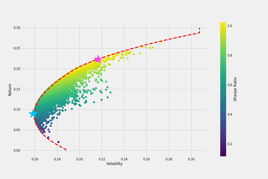
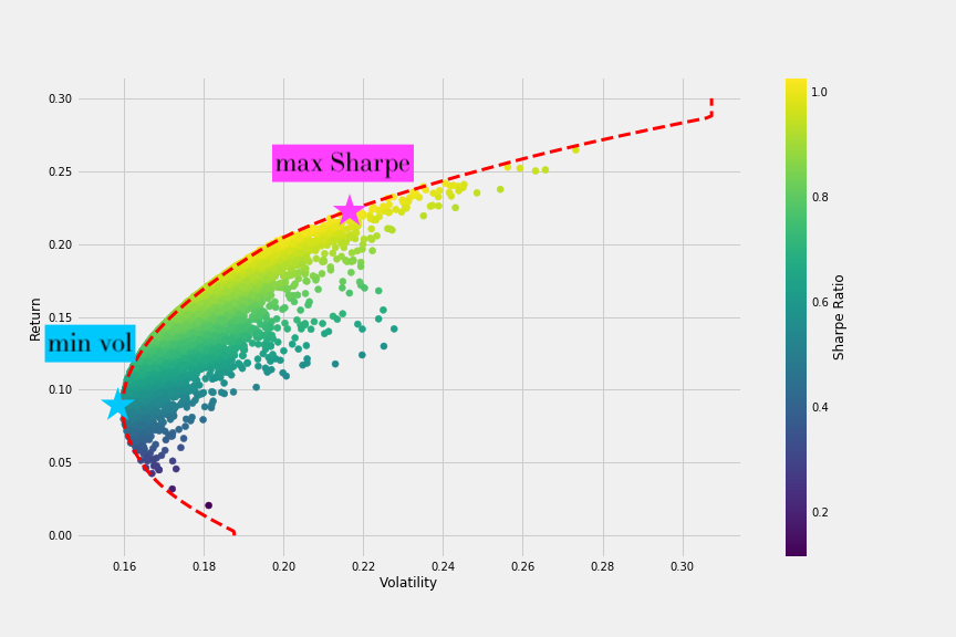
Portefeuille de Sharpe maximal : le ratio de Sharpe le plus élevé sur la FE
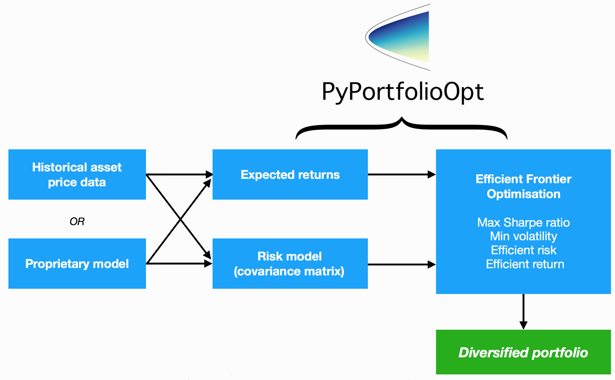
from pypfopt.efficient_frontier import EfficientFrontier
# Calculate the Efficient Frontier with mu and S
ef = EfficientFrontier(mu, Sigma)
raw_weights = ef.max_sharpe()
# Get interpretable weights
cleaned_weights = ef.clean_weights()
{'GOOG': 0.01269,'AAPL': 0.09202,'FB': 0.19856,
'BABA': 0.09642,'AMZN': 0.07158,'GE': 0.02456,...}
# Get performance numbers
ef.portfolio_performance(verbose=True)
Rendement annuel prévu : 33,0 %
Volatilité annuelle : 21,7 %
Ratio de Sharpe : 1,43
Portefeuille à volatilité minimale : le niveau de risque le plus bas sur la FE
# Calculate the Efficient Frontier with mu and S
ef = EfficientFrontier(mu, Sigma)
raw_weights = ef.min_volatility()
# Get interpretable weights and performance numbers
cleaned_weights = ef.clean_weights()
{'GOOG': 0.05664, 'AAPL': 0.087, 'FB': 0.1591,
'BABA': 0.09784, 'AMZN': 0.06986, 'GE': 0.0123,...}
ef.portfolio_performance(verbose=True)
Rendement annuel prévu : 17,4 %
Volatilité annuelle : 13,2 %
Ratio de Sharpe : 1,28


Introduction à l'analyse de portefeuille en Python