Introduction à l'analyse de portefeuille en Python
Charlotte Werger
Data Scientist

Voici Harry Markowitz

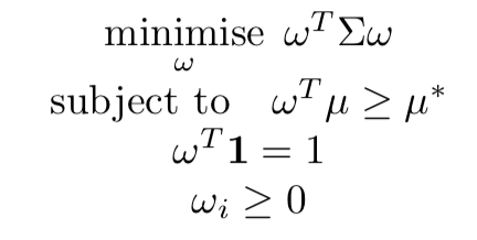
$$

En mots :

from pypfopt.efficient_frontier import EfficientFrontier
from pypfopt import risk_models
from pypfopt import expected_returns
df=pd.read_csv('portfolio.csv')
df.head(2)
XOM RRC BBY MA PFE
date
2010-01-04 54.068794 51.300568 32.524055 22.062426 13.940202
2010-01-05 54.279907 51.993038 33.349487 21.997149 13.741367
# Calculate expected annualized returns and sample covariance
mu = expected_returns.mean_historical_return(df)
Sigma = risk_models.sample_cov(df)
# Calculate expected annualized returns and risk
mu = expected_returns.mean_historical_return(df)
Sigma = risk_models.sample_cov(df)
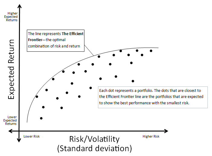
# Obtain the EfficientFrontier
ef = EfficientFrontier(mu, Sigma)
# Select a chosen optimal portfolio
ef.max_sharpe()
# Select the maximum Sharpe portfolio
ef.max_sharpe()
# Select an optimal return for a target risk
ef.efficient_risk(2.3)
# Select a minimal risk for a target return
ef.efficient_return(1.5)
# Obtain the performance numbers
ef.portfolio_performance(verbose=True, risk_free_rate = 0.01)
Rendement annuel espéré : 21,3 %
Volatilité annuelle : 19,5 %
Ratio de Sharpe : 0,98
Introduction à l'analyse de portefeuille en Python