Régression harmonique dynamique
Prévision en R

Rob J. Hyndman
Professor of Statistics at Monash University
Régression harmonique dynamique
Régression harmonique dynamique
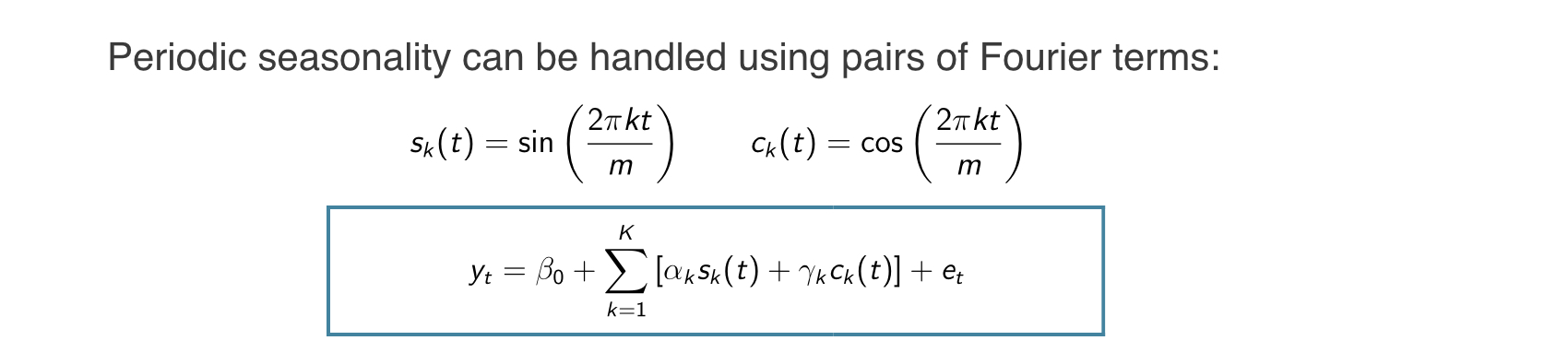
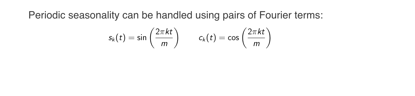
$m =$ période saisonnière
Toute fonction périodique peut être approchée par des sommes de termes sin et cos pour un K assez grand
Coefficients de régression : $\alpha_k$ et $\gamma_k$
$e_t$ peut être modélisé par un processus ARIMA non saisonnier
Suppose un profil saisonnier inchangé
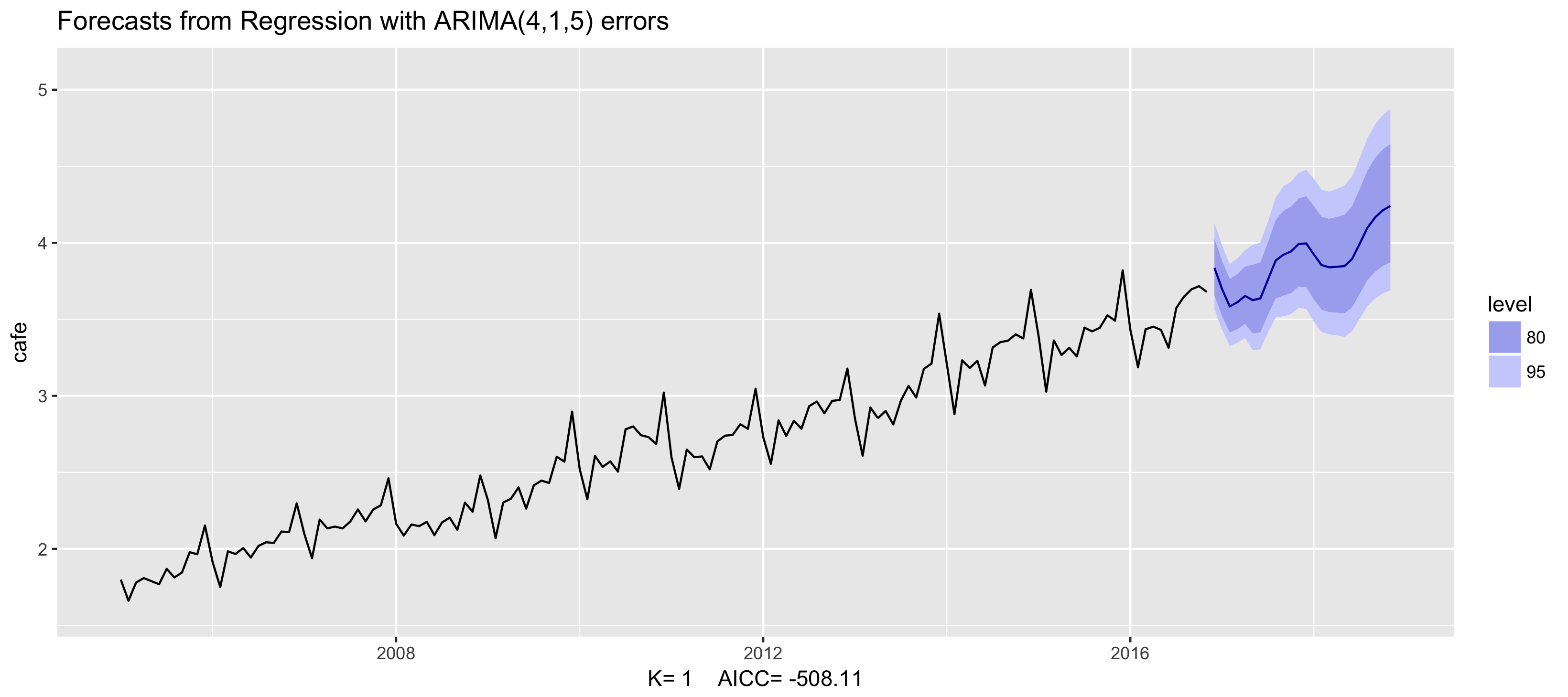
Exemple : dépenses dans les cafés australiens
fit <- auto.arima(cafe, xreg = fourier(cafe, K = 1),
                  seasonal = FALSE, lambda = 0)
fit %>% forecast(xreg = fourier(cafe, K = 1, h = 24)) %>%
   autoplot() + ylim(1.6, 5.1)
Exemple : dépenses dans les cafés australiens
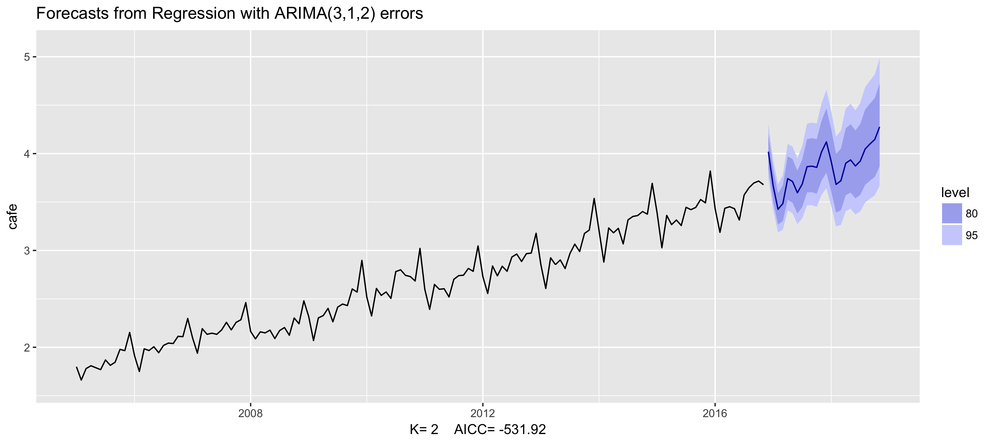
fit <- auto.arima(cafe, xreg = fourier(cafe, K = 2),
                  seasonal = FALSE, lambda = 0)
fit %>% forecast(xreg = fourier(cafe, K = 2, h = 24)) %>%
   autoplot() + ylim(1.6, 5.1)
Exemple : dépenses dans les cafés australiens
fit <- auto.arima(cafe, xreg = fourier(cafe, K = 3),
                  seasonal = FALSE, lambda = 0)
fit %>% forecast(xreg = fourier(cafe, K = 3, h = 24)) %>%
   autoplot() + ylim(1.6, 5.1)
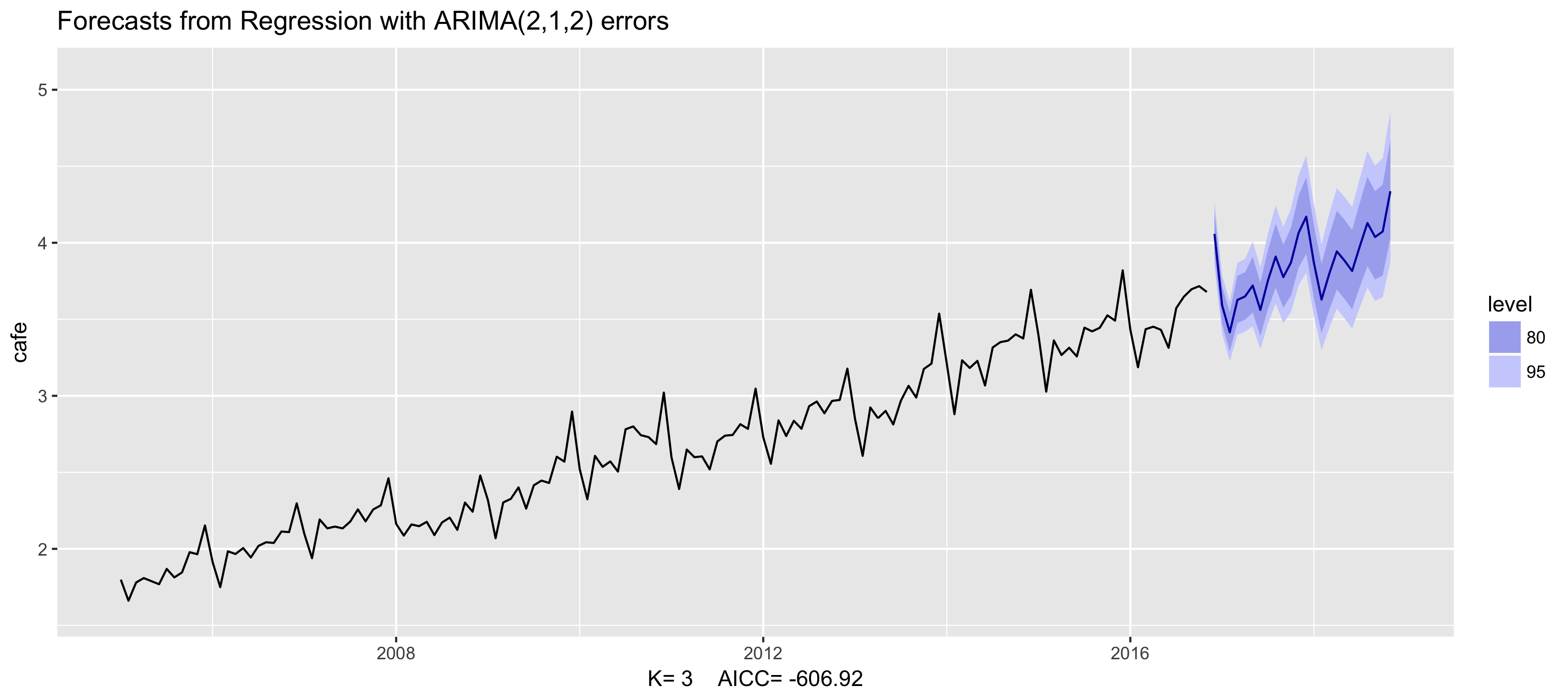
Exemple : dépenses dans les cafés australiens
fit <- auto.arima(cafe, xreg = fourier(cafe, K = 4),
                  seasonal = FALSE, lambda = 0)
fit %>% forecast(xreg = fourier(cafe, K = 4, h = 24)) %>%
   autoplot() + ylim(1.6, 5.1)
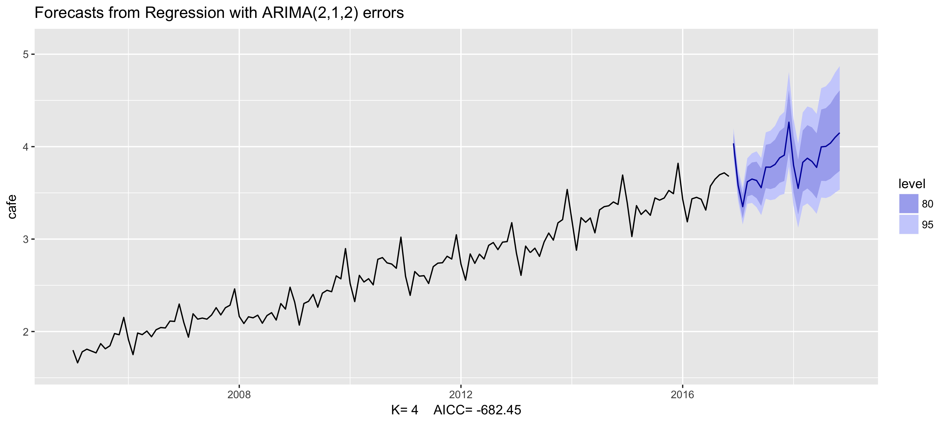
Exemple : dépenses dans les cafés australiens
fit <- auto.arima(cafe, xreg = fourier(cafe, K = 5),
                  seasonal = FALSE, lambda = 0)
fit %>% forecast(xreg = fourier(cafe, K = 5, h = 24)) %>%
   autoplot() + ylim(1.6, 5.1)
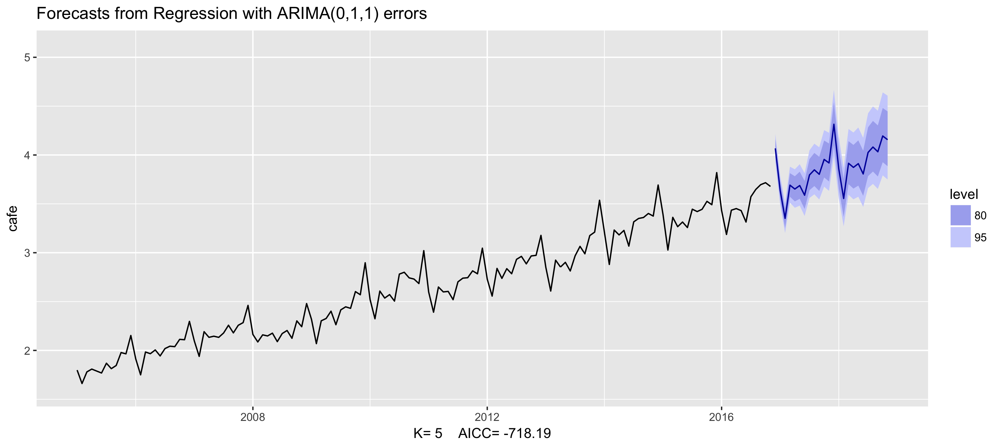
Exemple : dépenses dans les cafés australiens
fit <- auto.arima(cafe, xreg = fourier(cafe, K = 6),
                  seasonal = FALSE, lambda = 0)
fit %>% forecast(xreg = fourier(cafe, K = 6, h = 24)) %>%
   autoplot() + ylim(1.6, 5.1)
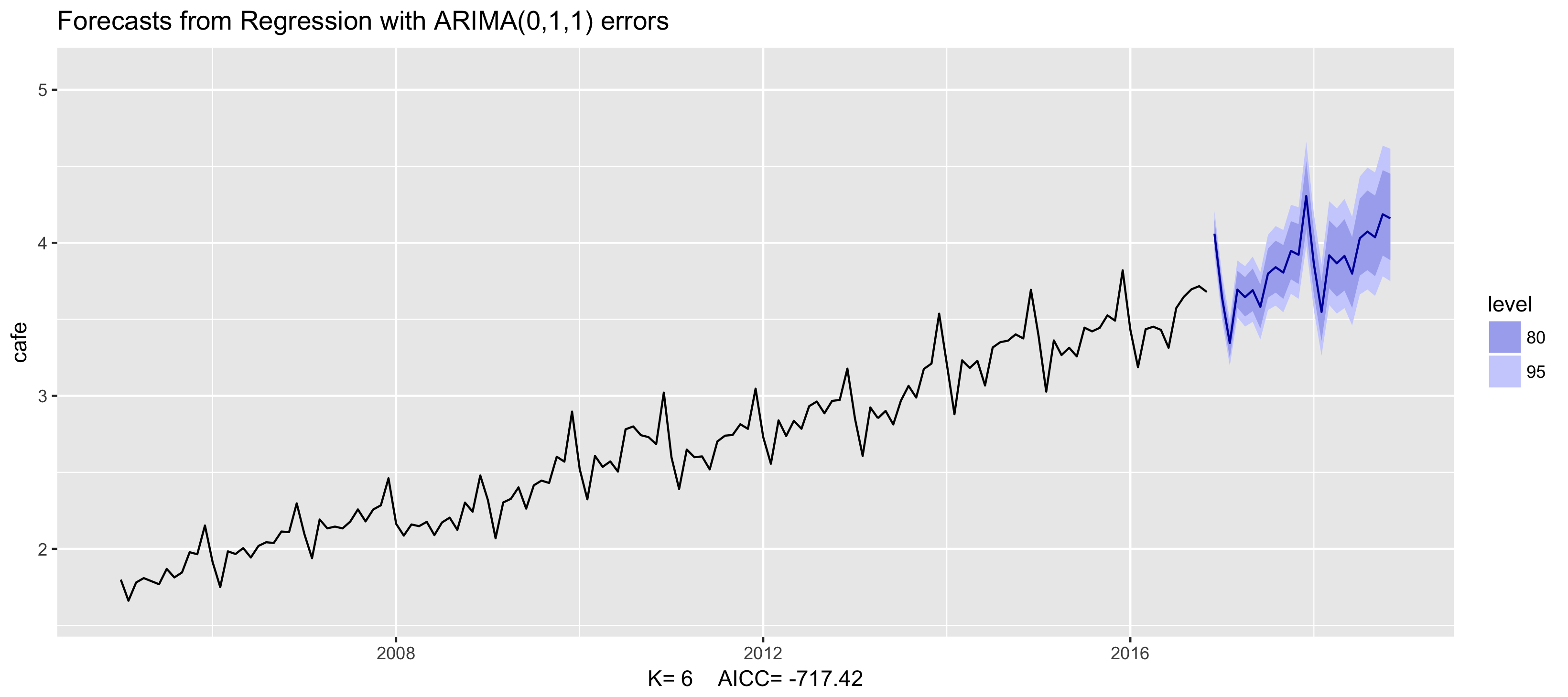
Régression harmonique dynamique

- D'autres variables prédictives peuvent aussi être ajoutées : $x_{t,1},...,x_{t,r}$
- Choisir K pour minimiser le $AIC_c$
- K ne peut pas dépasser m/2
- Particulièrement utile pour des données hebdomadaires, quotidiennes et infraquotidiennes

