Prévisions à pondération exponentielle

Prévision en R

Rob J. Hyndman

Professor of Statistics at Monash University

Lissage exponentiel simple

Notation des prévisions : $\hat y_{t + h \vert t} = \text{ prévision ponctuelle de } \ \hat y_{t + h} \ \text{ étant donné les données }\ y_1,...,y_t$

Équation de prévision : $\hat y_{t + h \vert t} = \alpha y_t + \alpha (1-\alpha ) y_{t-1} + \alpha (1-\alpha )^2 y_{t-2} +...$

$$où \ 0 \leq \alpha \leq 1 $$

Lissage exponentiel simple

Observation	$\alpha$ = 0.2	$\alpha$ = 0.4	$\alpha$ = 0.6	$\alpha$ = 0.8
$y_t$	0.2	0.4	0.6	0.8
$y_{t-1}$	0.16	0.24	0.24	0.16
$y_{t-2}$	0.128	0.144	0.096	0.032
$y_{t-3}$	0.1024	0.0864	0.0384	0.0064
$y_{t-4}$	(0.2)(0.8)$^4$	(0.4)(0.6)$^4$	(0.6)(0.4)$^4$	(0.8)(0.2)$^4$
$y_{t-5}$	(0.2)(0.8)$^5$	(0.4)(0.6)$^5$	(0.6)(0.4)$^5$	(0.8)(0.2)$^5$

Lissage exponentiel simple

Forme par composantes
Équation de prévision	$\hat{y}_{t+h \mid t} = \ell_t$
Équation de lissage	$\ell_t = \alpha y_t + (1-\alpha)\ell_{t-1}$

$\ell_t \ $ est le niveau (ou la valeur lissée) de la série au temps $t$
On choisit $\alpha$ et $\ell_0$ en minimisant la SSE :

$$SSE = \sum_{t=1}^T (y_t - \hat y_{t\vert t-1})^2$$

Exemple : production de pétrole

oildata <- window(oil, start = 1996)    # Données pétrolières
fc <- ses(oildata, h = 5)               # Lissage exponentiel simple
summary(fc)

Méthode de prévision : lissage exponentiel simple
Renseignements sur le modèle :
Lissage exponentiel simple
Appel :
 ses(y = oildata, h = 5)
  Paramètres de lissage :
    alpha = 0.8339
  États initiaux :
    l = 446.5759
  sigma :  28.12
*** Tronqué par manque d'espace

Exemple : production de pétrole

autoplot(fc) +
  ylab("Pétrole (millions de tonnes)") + xlab("Année")

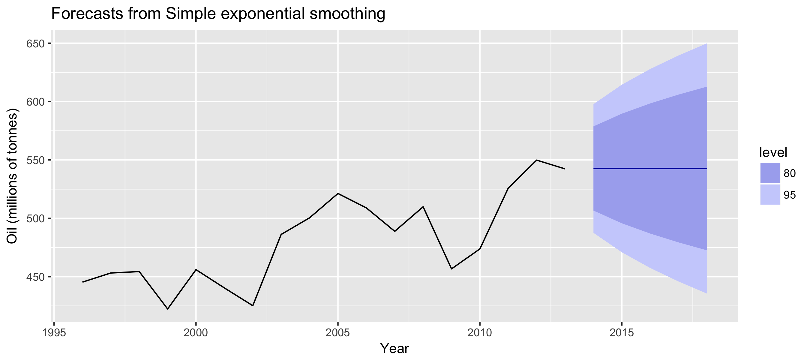
Production pétrolière : lissage exponentiel simple

Passons à la pratique !

Prévision en R