Lissage exponentiel avec tendance

Prévision en R

Rob J. Hyndman

Professor of Statistics at Monash University

Tendance linéaire de Holt

Lissage exponentiel simple
Prévision $\hat{y}_{t+h \mid t} = \ell_t$
Niveau $\ell_t = \alpha y_t + (1-\alpha)\ell_{t-1}$


Tendance linéaire de Holt
Prévision $\hat{y}_{t+h \mid t} = \ell_t + hb_t$
Niveau $\ell_t = \alpha y_t + (1-\alpha)(\ell_{t-1} + b_{t-1})$
Tendance $b_t = \beta^*(\ell_t = \ell_{t-1}) + (1 - \beta^*) b_{t-1}$
Prévision en R

Tendance linéaire de Holt

Tendance linéaire de Holt
Prévision $\hat{y}_{t+h \mid t} = \ell_t + hb_t$
Niveau $\ell_t = \alpha y_t + (1-\alpha)(\ell_{t-1} + b_{t-1})$
Tendance $b_t = \beta^*(\ell_t = \ell_{t-1}) + (1 - \beta^*) b_{t-1}$


  • Deux paramètres de lissage $\alpha$ et $\beta^*$ avec $0 \leq \alpha$ et $\beta^* \leq 1$

  • Choisir $\alpha, \beta^*, \ell_0, b_0$ pour minimiser la SSE

Prévision en R

Méthode de Holt en R

airpassengers %>% holt(h = 5) %>% autoplot
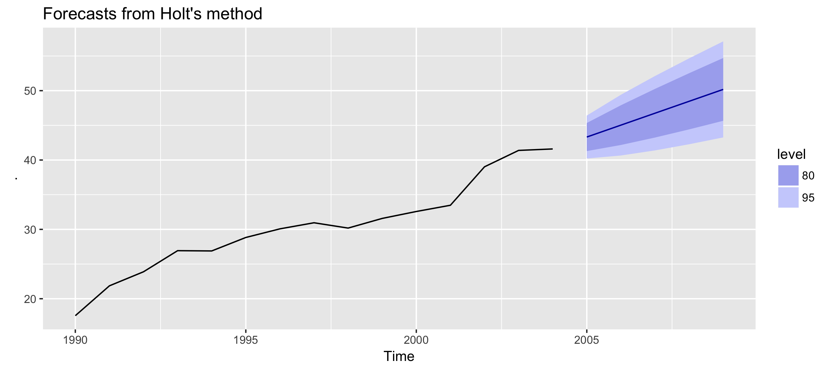
ch3_vid2_holt.png

Prévision en R

Méthode à tendance amortie

Forme par composantes
$\hat{y}_{t+h \mid t} = \ell_t + (\phi + \phi^2 + ... + \phi^h)b_t$
$\ell_t = \alpha y_t + (1-\alpha)(\ell_{t-1} + \phi b_{t-1})$
$b_t = \beta^*(\ell_t = \ell_{t-1}) + (1 - \beta^*) \phi b_{t-1}$


  • Paramètre d'amortissement $\ 0 < \phi < 1$
  • Si $\ \phi = 1$, identique à la tendance linéaire de Holt
  • Prévisions à court terme avec tendance, à long terme constantes
Prévision en R

Exemple : passagers aériens

fc1 <- holt(airpassengers, h = 15, PI = FALSE)
fc2 <- holt(airpassengers, damped = TRUE, h = 15, PI = FALSE)
autoplot(airpassengers) + xlab("Year") + ylab("millions") +
  autolayer(fc1, series="Linear trend") +
  autolayer(fc2, series="Damped trend")
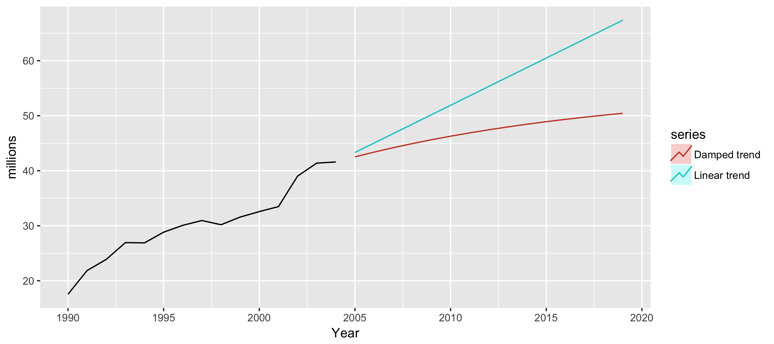
ch3_vid2_damp.png

Prévision en R

Passons à la pratique !

Prévision en R

Preparing Video For Download...