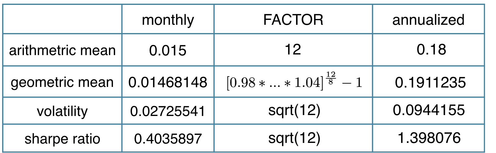
Le ratio de Sharpe (annualisé)
Introduction à l'analyse de portefeuille en R

Kris Boudt
Professor, Free University Brussels & Amsterdam
Évaluer la performance par rapport à un étalon
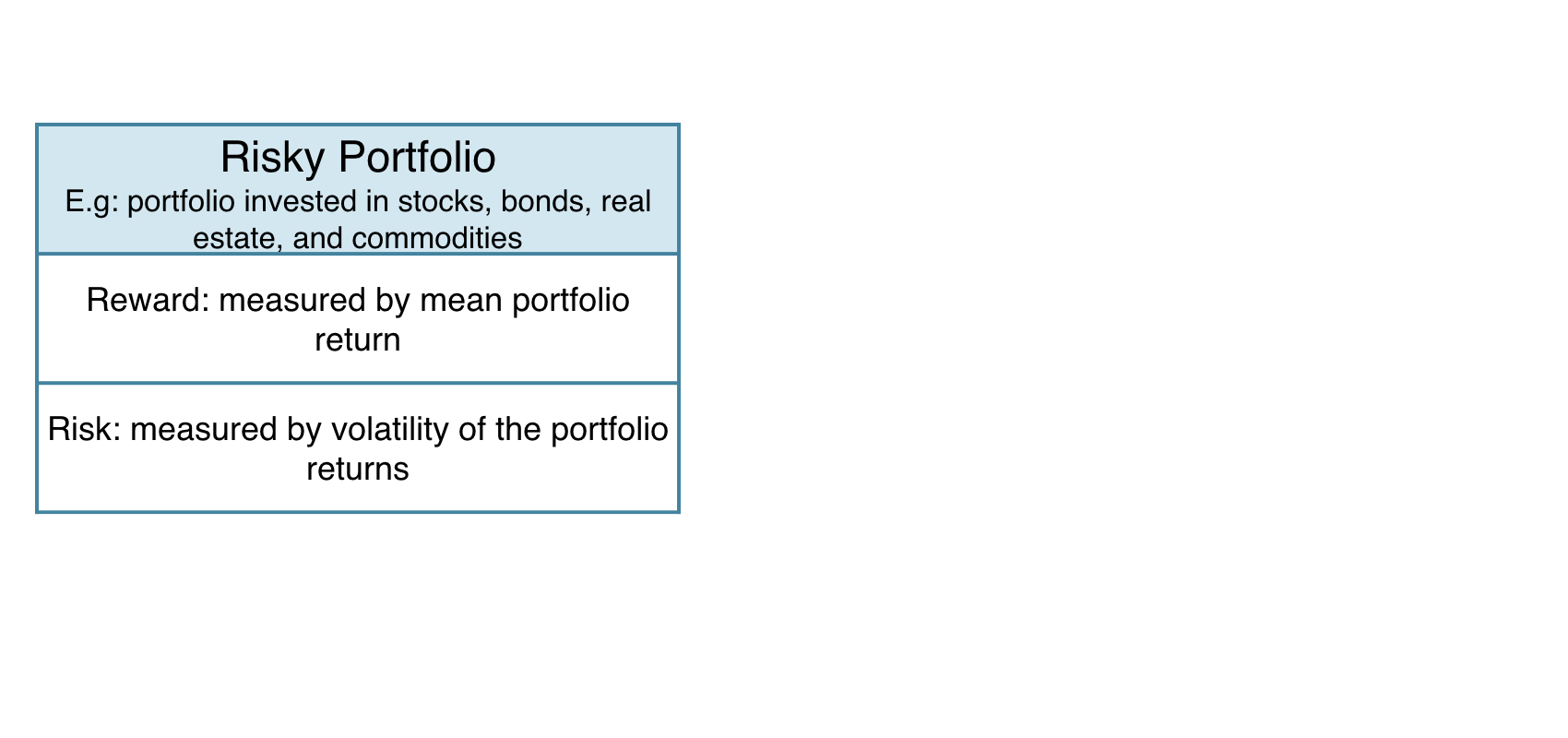
Évaluer la performance par rapport à un étalon
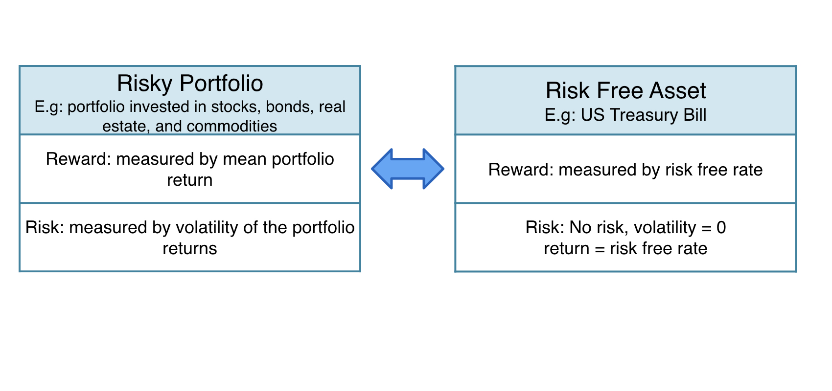
Le compromis risque-rendement
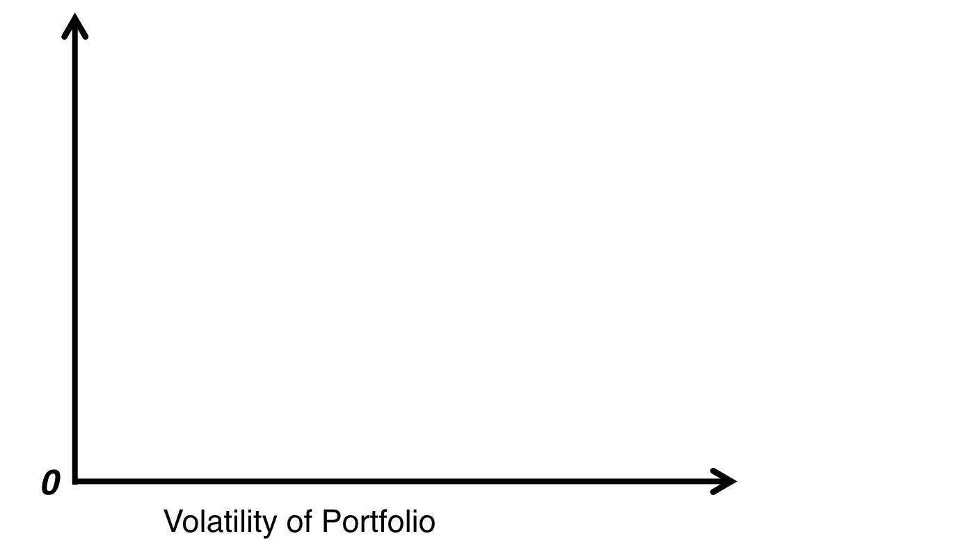
Le compromis risque-rendement
Le compromis risque-rendement
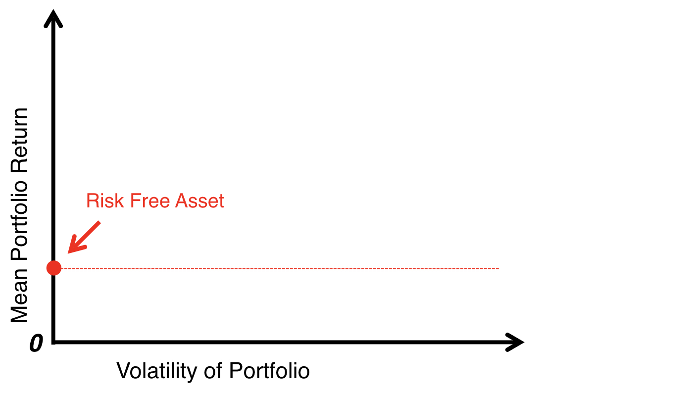
Le compromis risque-rendement
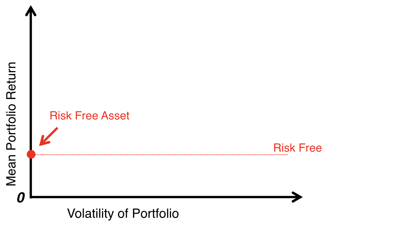
Le compromis risque-rendement
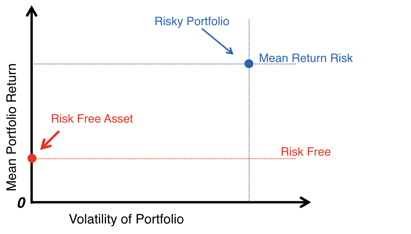
Le compromis risque-rendement
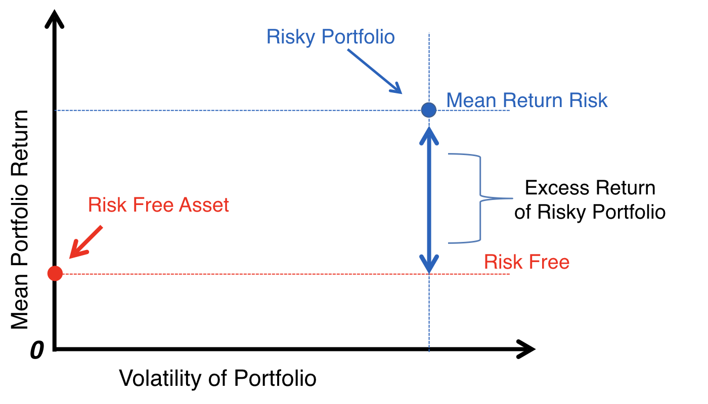
Droite d'allocation du capital
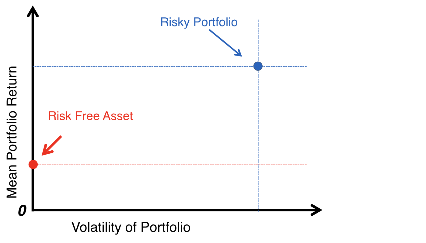
Droite d'allocation du capital
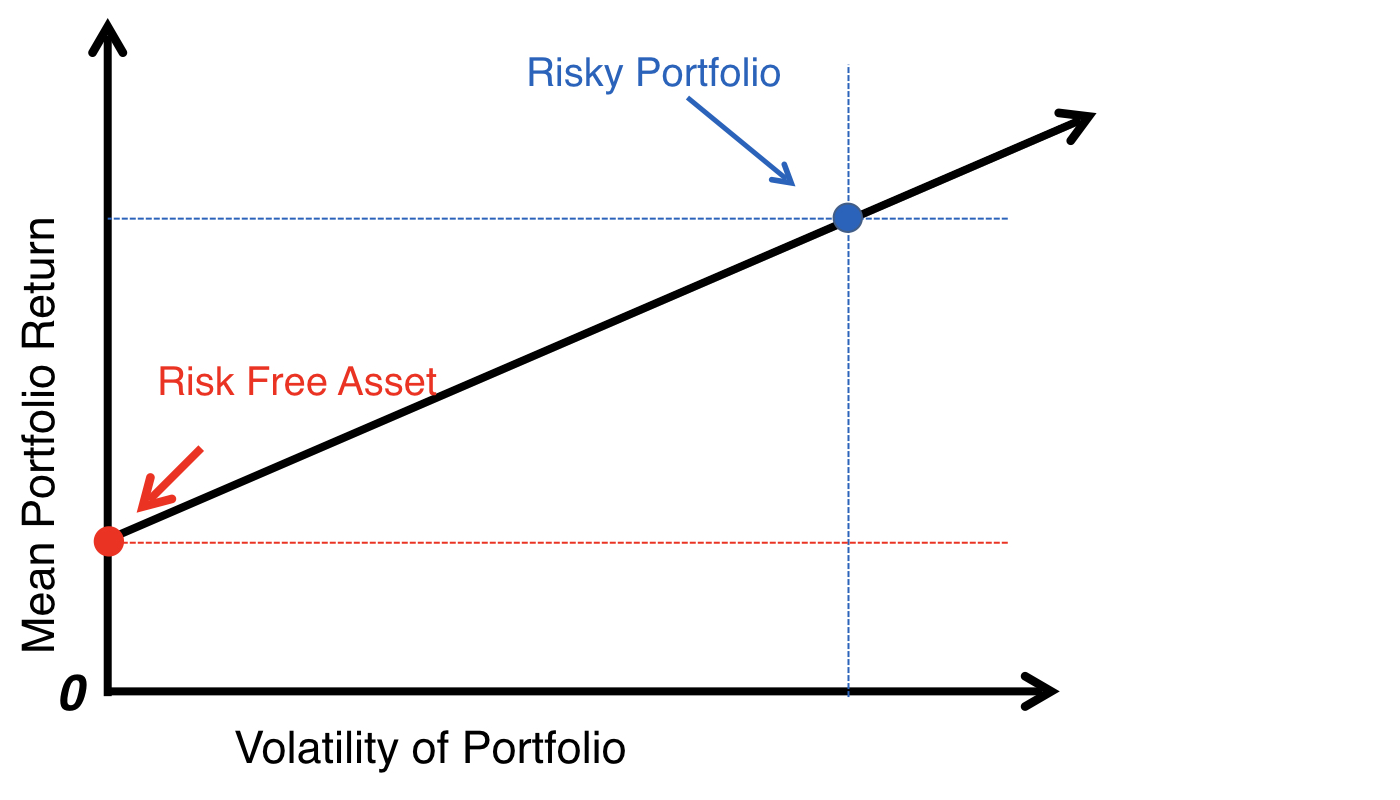
Droite d'allocation du capital
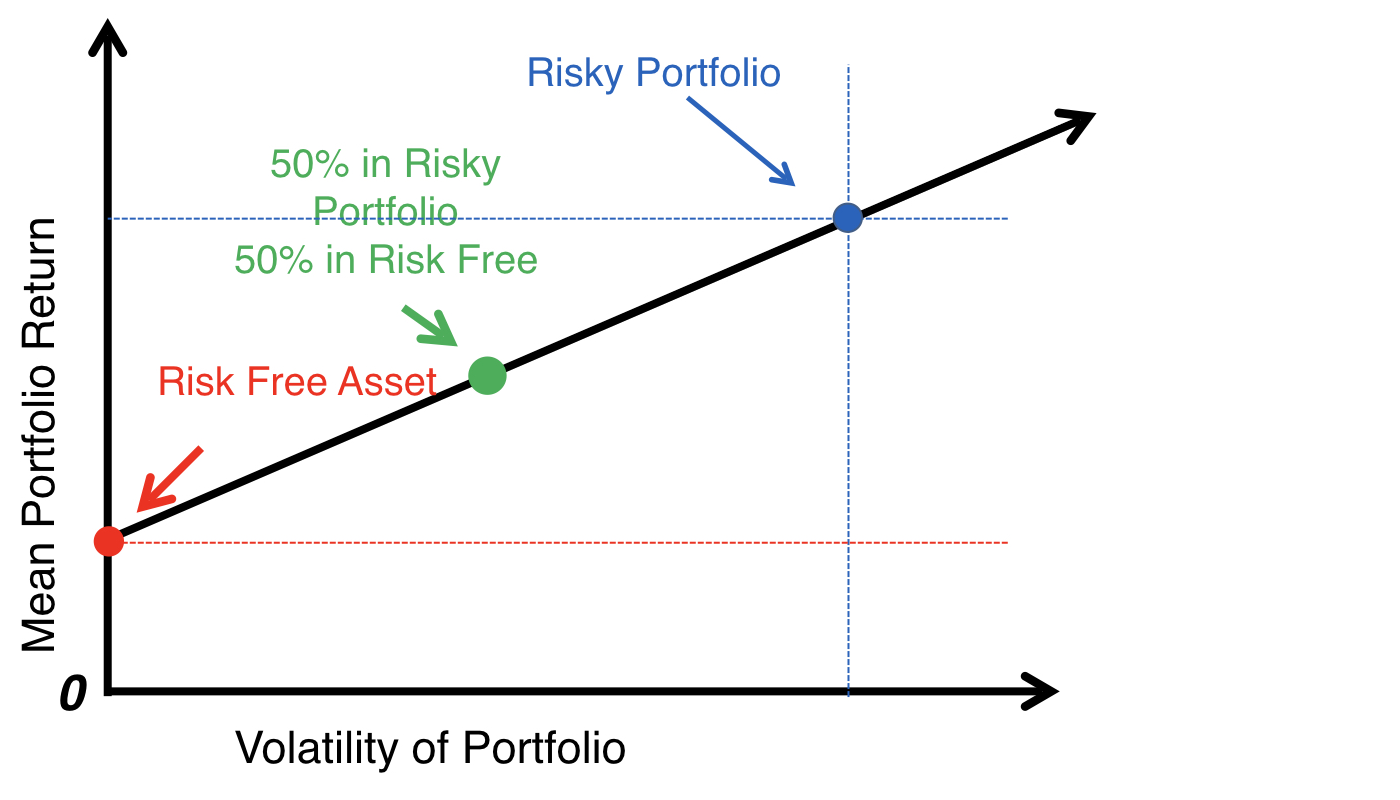
Droite d'allocation du capital
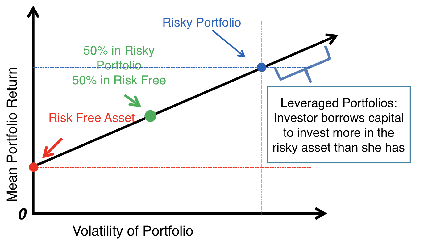
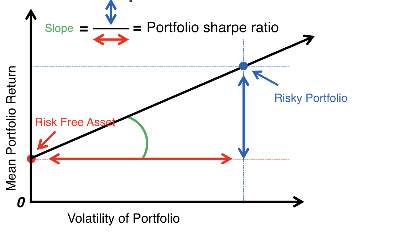
Le ratio de Sharpe
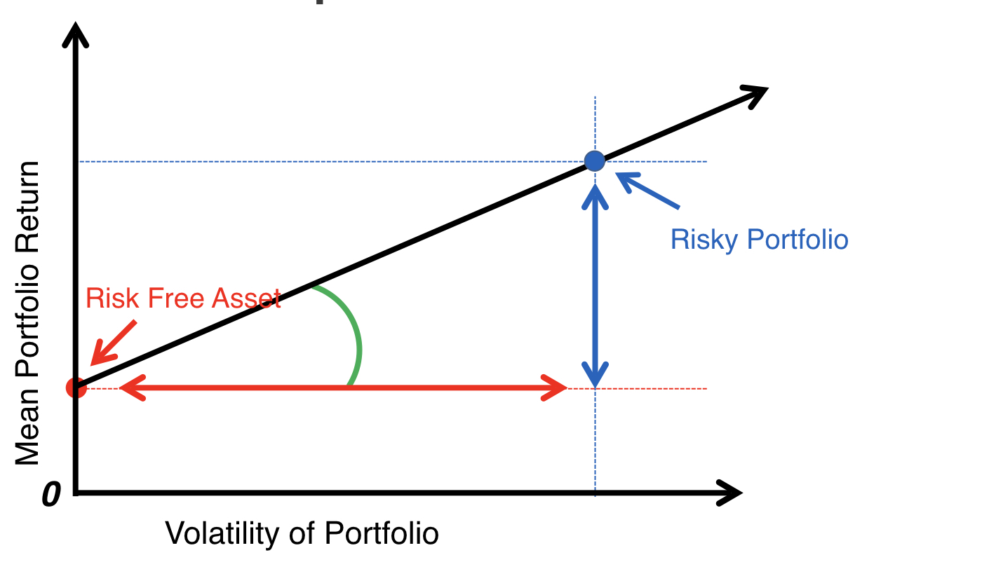
Le ratio de Sharpe
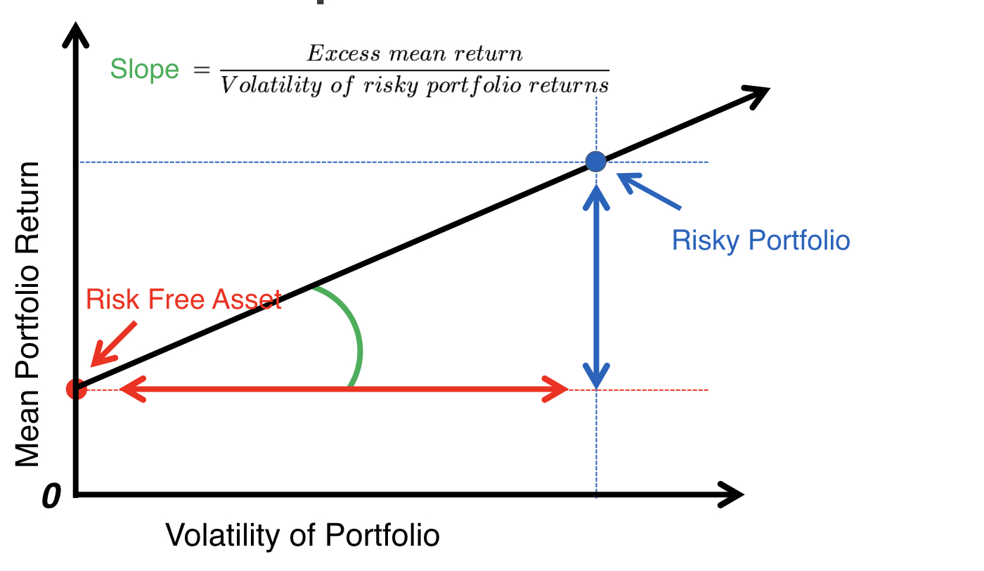
Le ratio de Sharpe
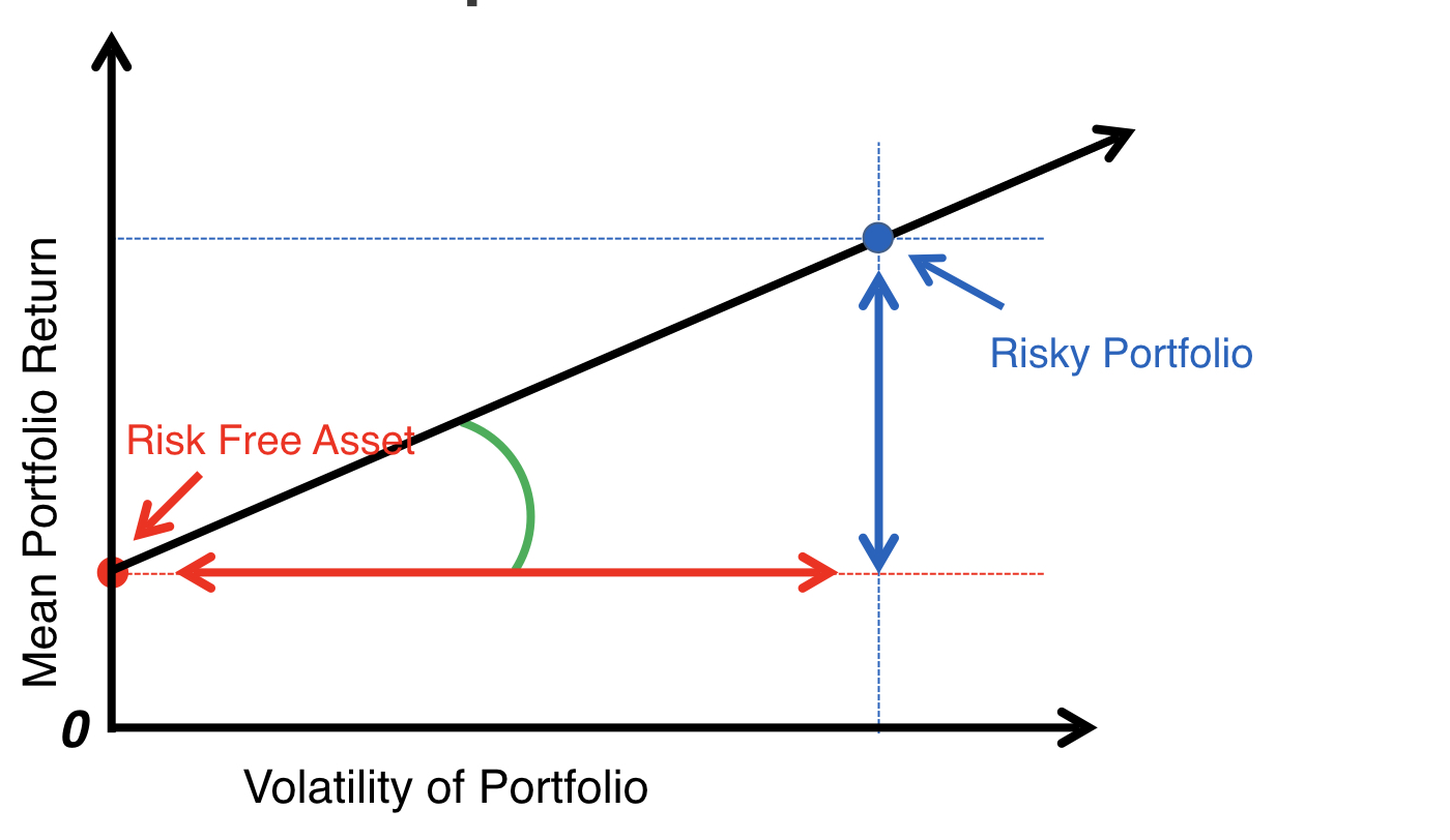
Le ratio de Sharpe
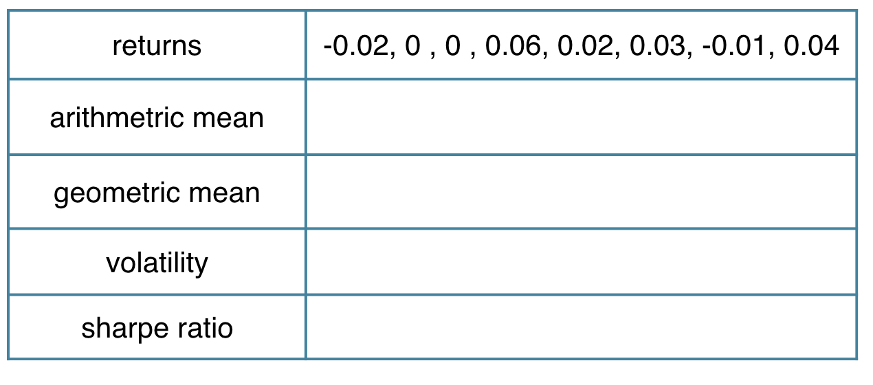
Statistiques de performance en action
library(PerformanceAnalytics)
sample_returns <- c(-0.02, 0.00, 0.00, 0.06, 0.02, 0.03, -0.01, 0.04)
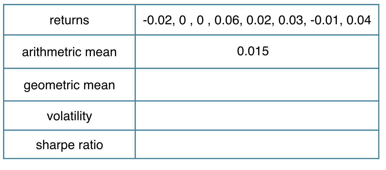
Statistiques de performance en action
library(PerformanceAnalytics)
sample_returns <- c(-0.02, 0.00, 0.00, 0.06, 0.02, 0.03, -0.01, 0.04)
mean(sample_returns)
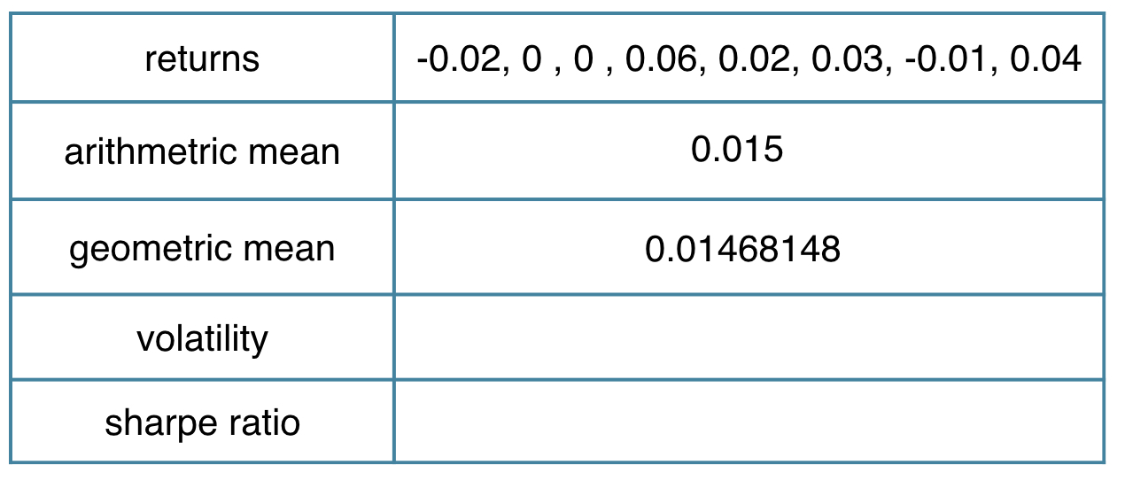
Statistiques de performance en action
library(PerformanceAnalytics)
sample_returns <- c(-0.02, 0.00, 0.00, 0.06, 0.02, 0.03, -0.01, 0.04)
mean.geometric(sample_returns)
Statistiques de performance en action
library(PerformanceAnalytics)
sample_returns <- c(-0.02, 0.00, 0.00, 0.06, 0.02, 0.03, -0.01, 0.04)
StdDev(sample_returns)
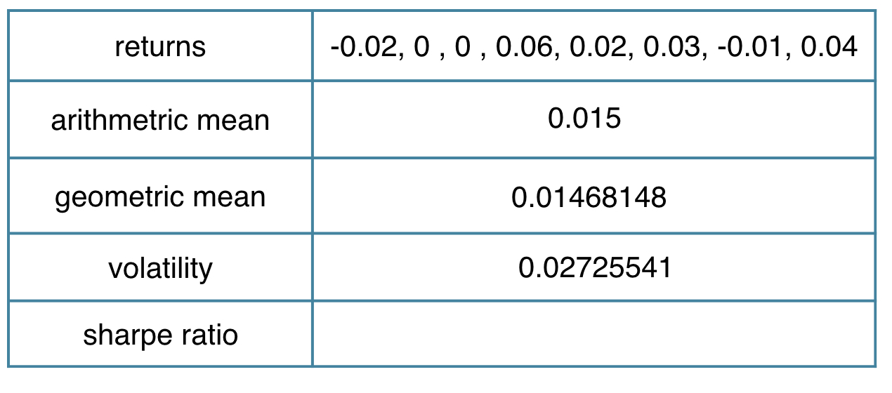
Statistiques de performance en action
library(PerformanceAnalytics)
sample_returns <- c(-0.02, 0.00, 0.00, 0.06, 0.02, 0.03, -0.01, 0.04)
(mean(sample_returns)-0.004)/StdDev(sample_returns)
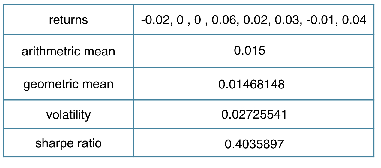
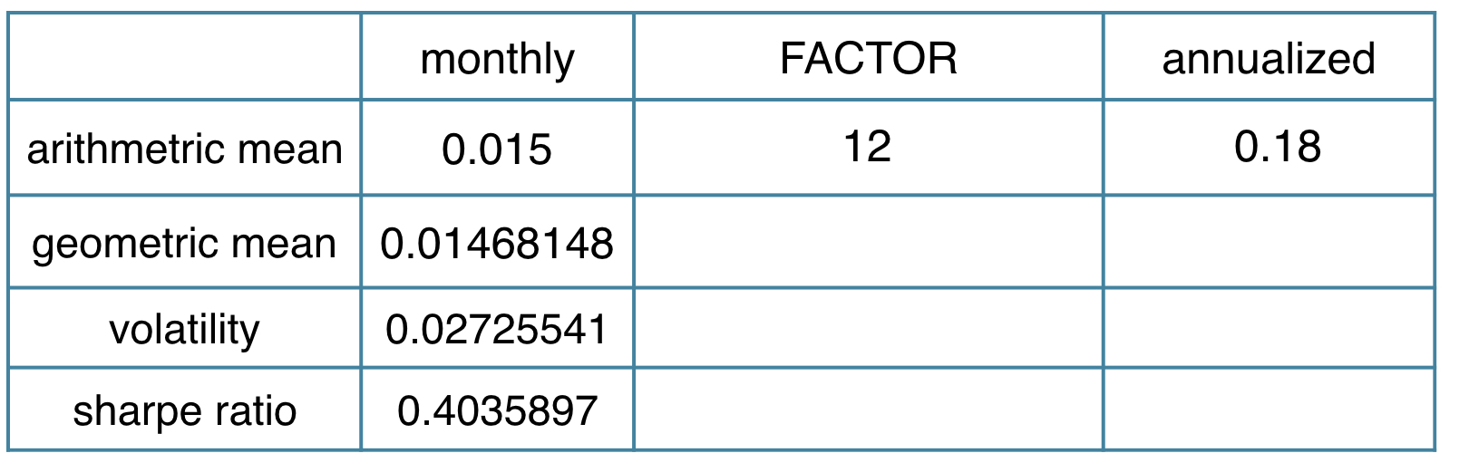
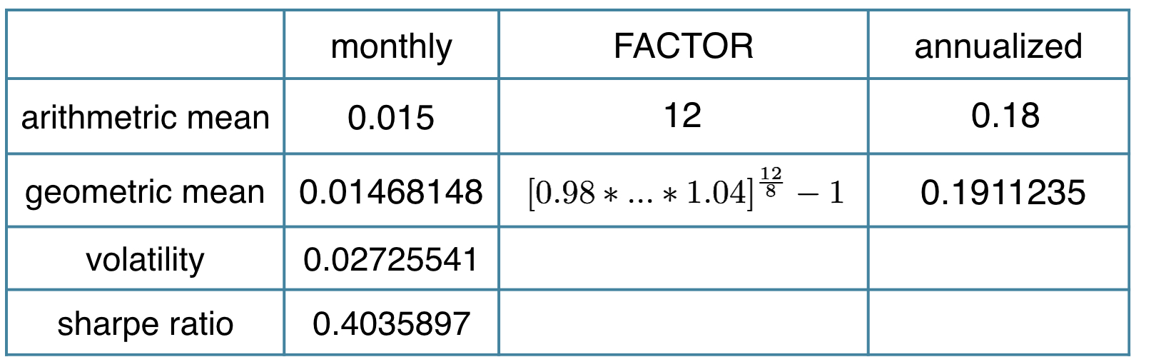
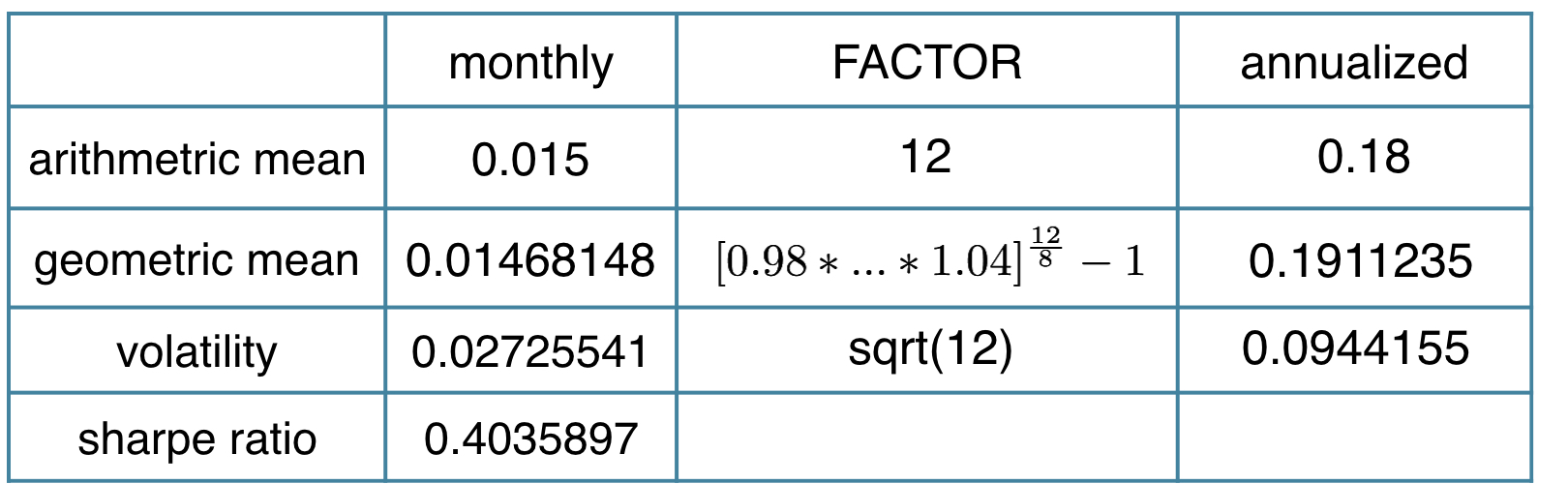
Annualiser la performance mensuelle
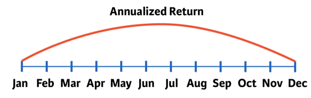
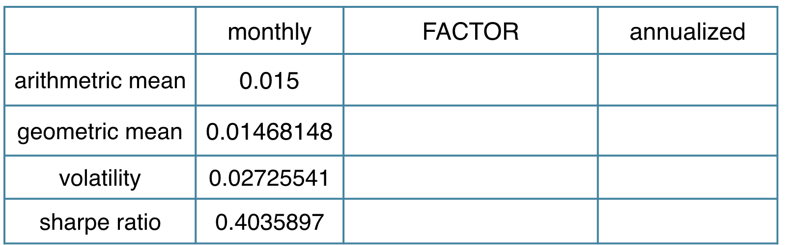
- Moyenne arithmétique : moyenne mensuelle * 12
- Moyenne géométrique, si $R_i$ sont des rendements mensuels :
- $[(1+R_1)\cdot(1+R_2)\cdot...\cdot(1+R_T)]^{12/T} -1$
- Volatilité : volatilité mensuelle * sqrt(12)
Statistiques de performance en action
library(PerformanceAnalytics)
sample_returns <- c( -0.02, 0.00, 0.00, 0.06, 0.02, 0.03, -0.01, 0.04)
Statistiques de performance en action
library(PerformanceAnalytics)
sample_returns <- c( -0.02, 0.00, 0.00, 0.06, 0.02, 0.03, -0.01, 0.04)
Return.annualized(sample_returns, scale = 12, geometric = FALSE)
Statistiques de performance en action
library(PerformanceAnalytics)
sample_returns <- c( -0.02, 0.00, 0.00, 0.06, 0.02, 0.03, -0.01, 0.04)
Return.annualized(sample_returns, scale = 12, geometric = TRUE)
Statistiques de performance en action
library(PerformanceAnalytics)
sample_returns <- c( -0.02, 0.00, 0.00, 0.06, 0.02, 0.03, -0.01, 0.04)
Std.Dev.annualized(sample_returns, scale = 12)
Statistiques de performance en action
library(PerformanceAnalytics)
sample_returns <- c( -0.02, 0.00, 0.00, 0.06, 0.02, 0.03, -0.01, 0.04)
Return.annualized(sample_returns, scale = 12)/
    Std.Dev.annualized(sample_returns, scale = 12)