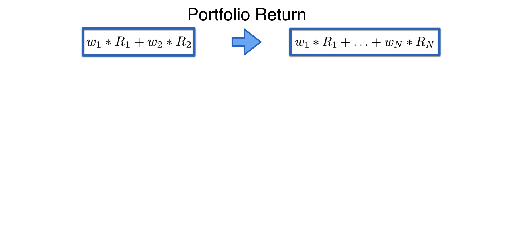
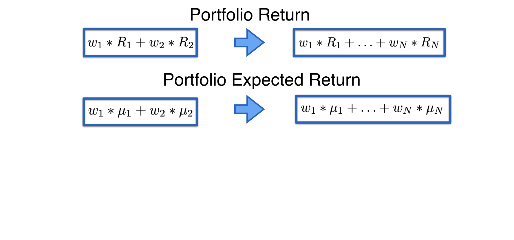
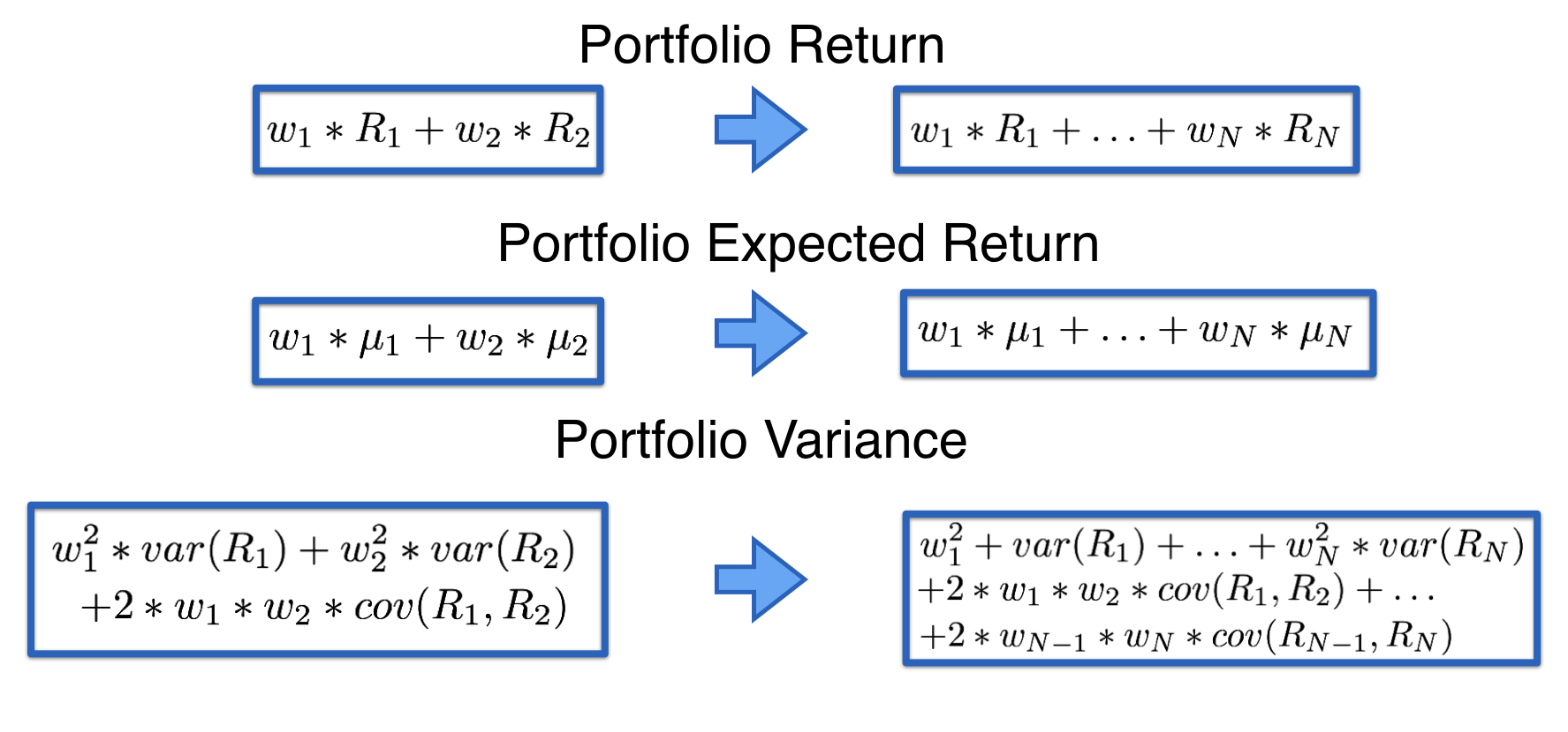
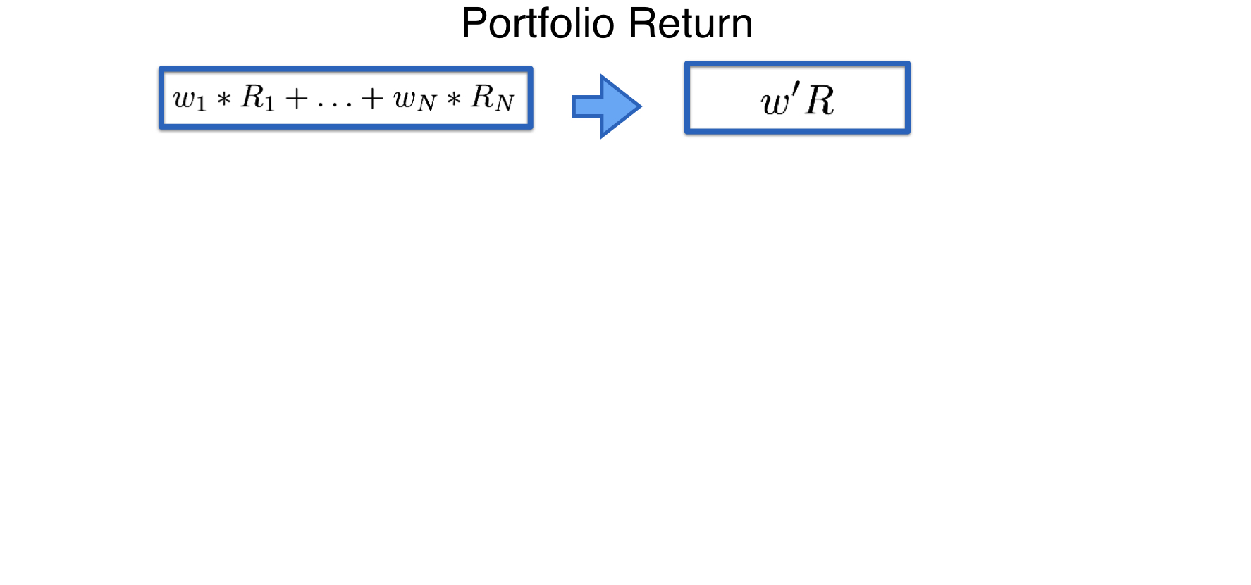
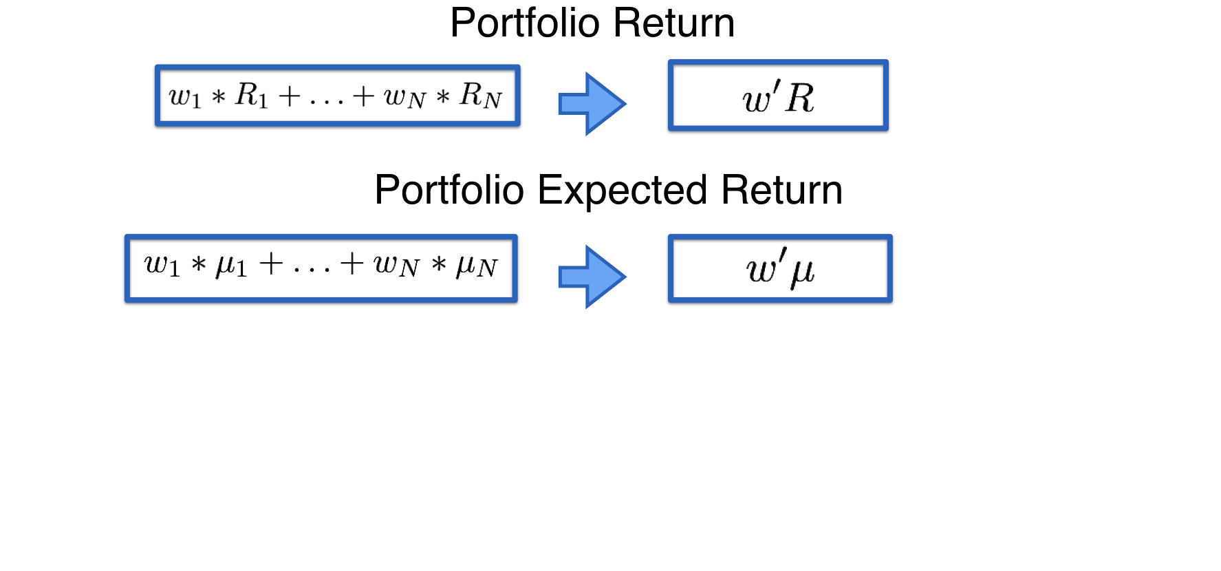
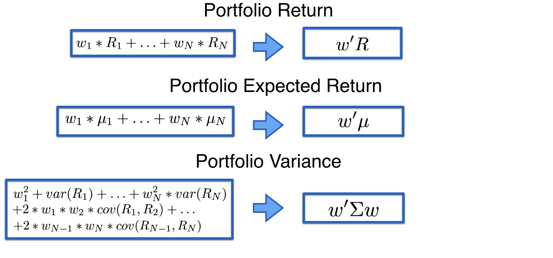
Variables en jeu pour n actifs
$w$ : matrice colonne $N$ x 1 des pondérations du portefeuille :
$$w = \left[{\begin{array}{c} w_1 \\ w_2 \\ ...\\w_N\end{array} }\right]$$
$\mu$ : matrice colonne $N$ x 1 des rendements attendus :
$$\mu = \left[{\begin{array}{c} \mu_1 \\ \mu_2 \\ ...\\ \mu_N\end{array} }\right]$$
$R$ : matrice colonne $N$ x 1 des rendements des actifs :
$$ \color{red} {R =\left[{\begin{array}{c} R_1 \\ R_2 \\ ...\\R_N\end{array} }\right]}$$
$\Sigma$ : matrice de covariance $N$ x $N$ des $N$ rendements d'actifs :
$$w = \left[
{\begin{array}{cccc}
{\large \sigma^2_{1}} & \sigma_{12} & ... & \sigma_{1N} \\
\sigma_{21} & {\large \sigma^2_{2}} & ... & \sigma_{2N} \\ ... & ... & ... & ... \\ \sigma_{N1} & \sigma_{N2} & ... & {\large \sigma^2_{N}}
\end{array} }
\right]$$