Choisir le bon nombre de composantes principales

Machine Learning for Marketing Analytics in R

Verena Pflieger

Data Scientist at INWT Statistics

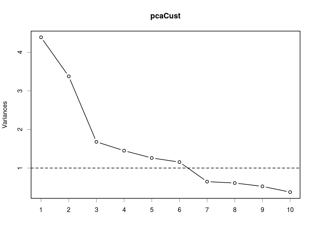
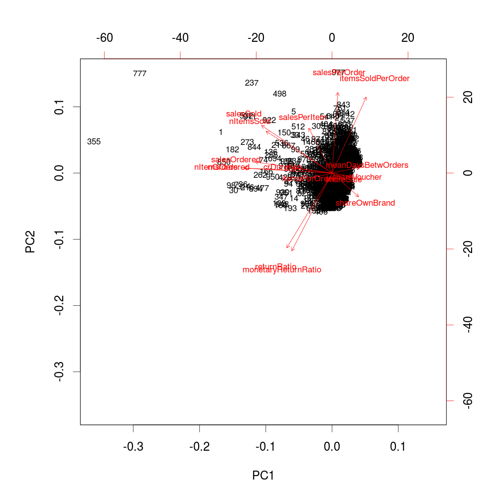
Nb de composantes pertinentes : variance expliquée

# Proportion de variance expliquée :
summary(pcaCust)

Importance of components:
                          PC1    PC2    PC3     PC4     PC5     PC6     PC7
Standard deviation     2.0951 1.8379 1.2960 1.20415 1.12301 1.07453 0.80486
Proportion of Variance 0.2743 0.2111 0.1050 0.09062 0.07882 0.07216 0.04049
Cumulative Proportion  0.2743 0.4855 0.5904 0.68106 0.75989 0.83205 0.87254
                           PC8     PC9    PC10    PC11    PC12    PC13
Standard deviation     0.78236 0.72452 0.61302 0.48428 0.36803 0.25901
Proportion of Variance 0.03826 0.03281 0.02349 0.01466 0.00847 0.00419
Cumulative Proportion  0.91079 0.94360 0.96709 0.98175 0.99021 0.99440
                          PC14    PC15    PC16
Standard deviation     0.20699 0.17126 0.13170
Proportion of Variance 0.00268 0.00183 0.00108
Cumulative Proportion  0.99708 0.99892 1.00000

Nb de composantes pertinentes : critère de Kaiser-Guttman

Critère de Kaiser-Guttman : valeur propre > 1

pcaCust$sdev ^ 2

 [1] 4.38961593 3.37778445 1.67965616 1.44997580 1.26115351 1.15461579
 [7] 0.64780486 0.61209376 0.52492468 0.37579685 0.23452736 0.13544710
[13] 0.06708362 0.04284504 0.02933027 0.01734481

Nb de composantes pertinentes : screeplot

Le screeplot ou : « trouver le coude »

screeplot(pcaCust, type = "lines")
box()
abline(h = 1, lty = 2)

Nombre suggéré de composantes par critère

Variance expliquée	Kaiser-Guttman	Screeplot
5	6	6

Le biplot

biplot(pcaCust, choices = 1:2, cex = 0.7)

Passons à la pratique !

Machine Learning for Marketing Analytics in R