Lois de probabilité multivariée en R
Surajit Ray
Professor, University of Glasgow
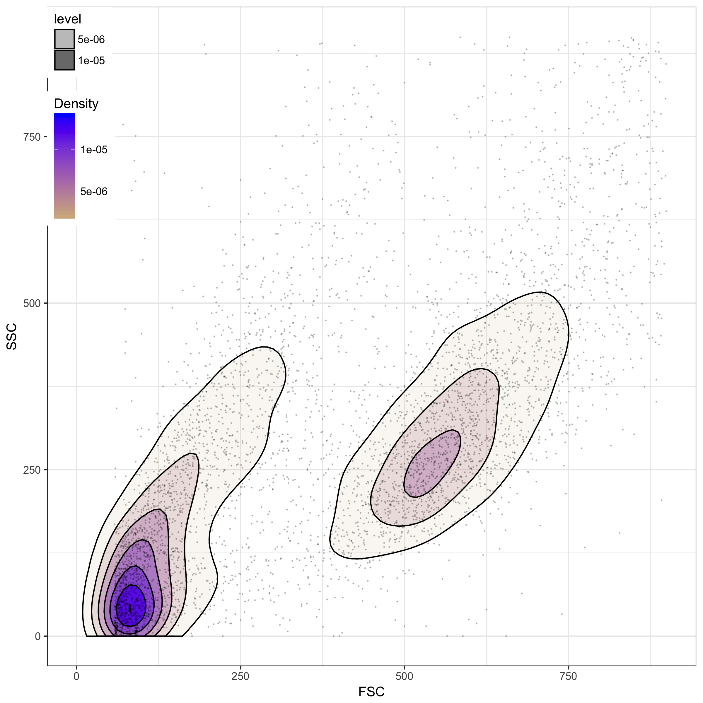
Données de cytométrie en flux — diffusion latérale (SSC) et diffusion avant (FSC)
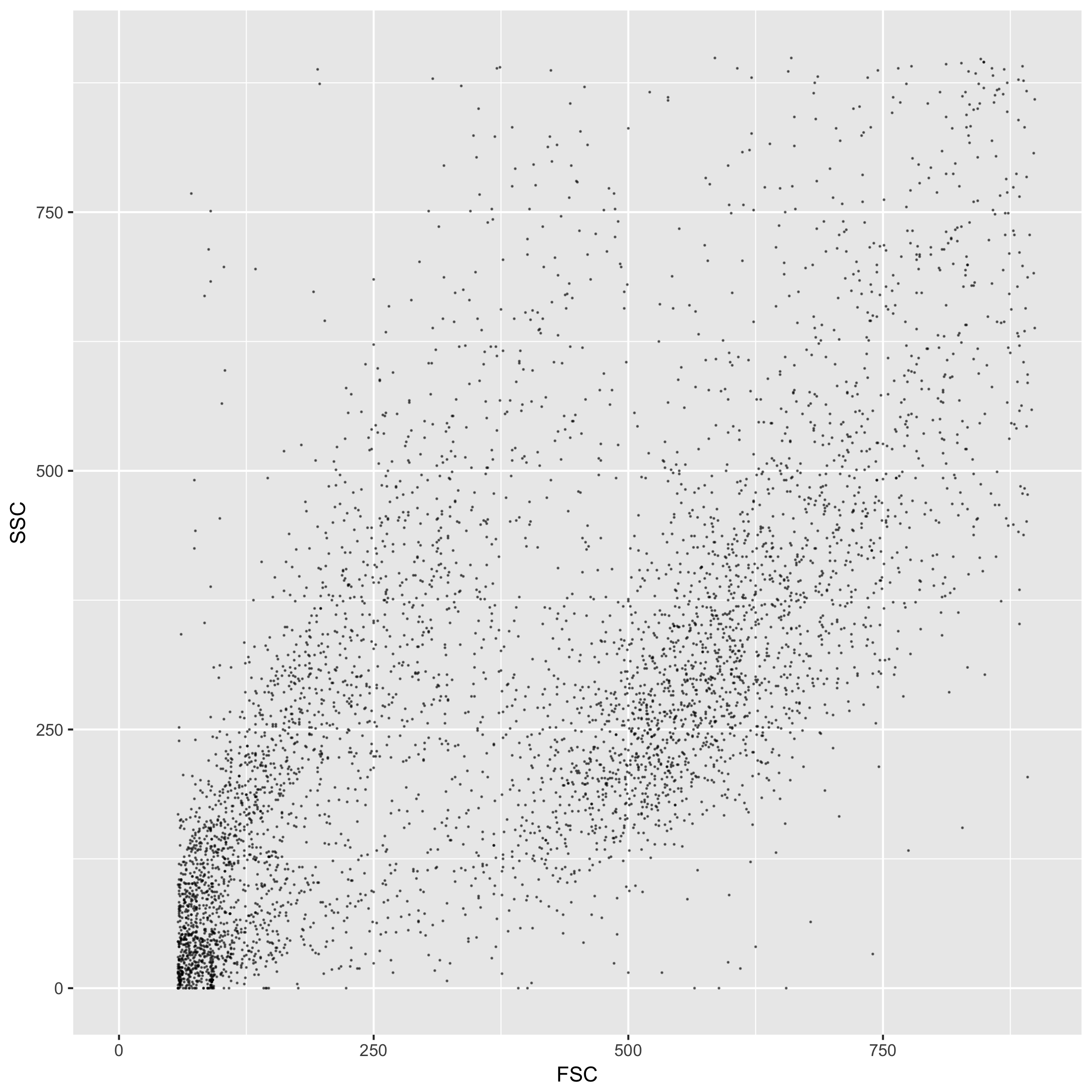
Données de cytométrie en flux — diffusion latérale (SSC) et diffusion avant (FSC)
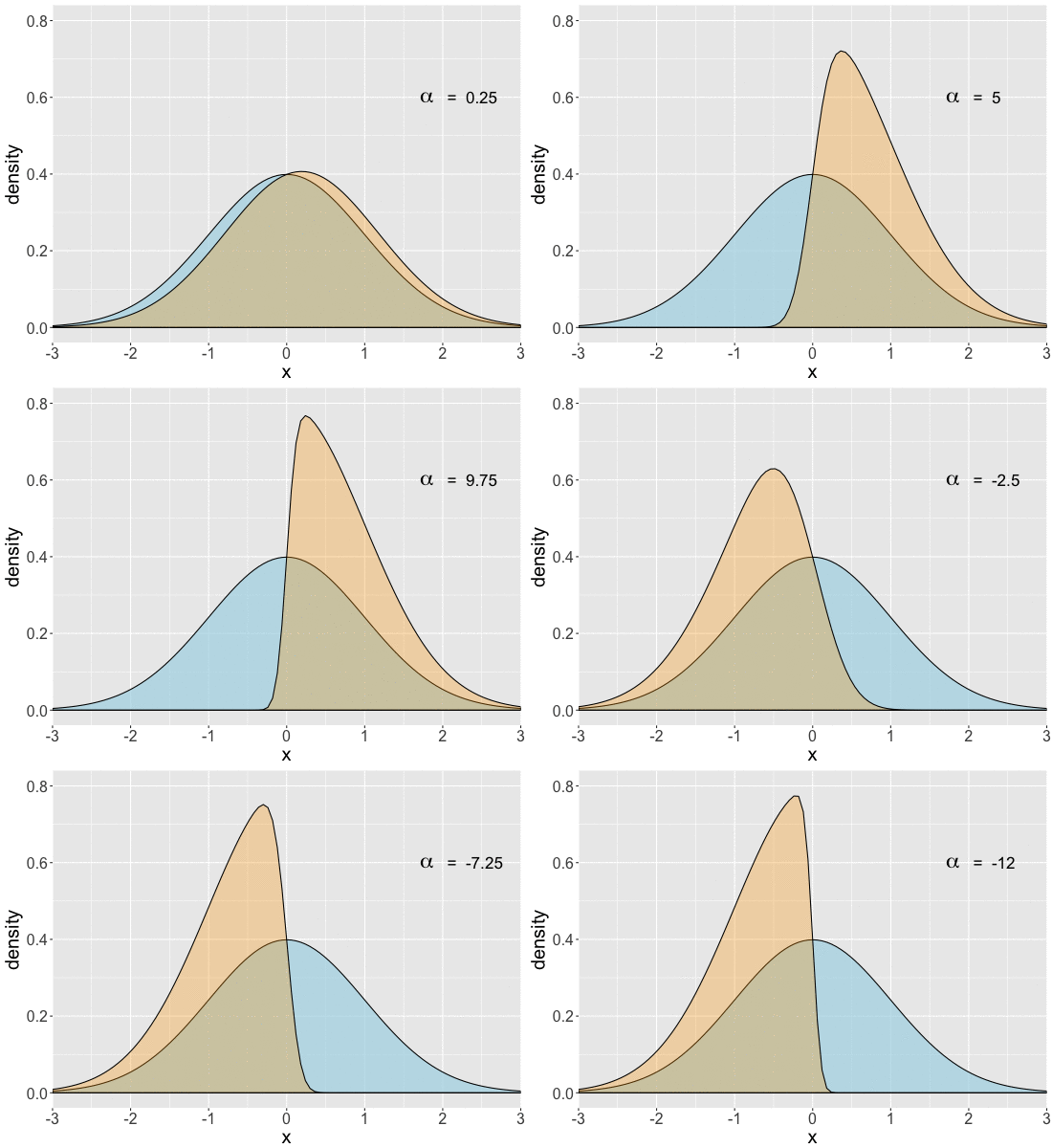
La loi normale asymétrique générale se note $SN(\xi,\omega,\alpha)$
Forme la plus simple : $z \sim SN(\alpha)$
Comparer $SN(\alpha)$ à une normale standard
Notations : distribution normale asymétrique multivariée en trois dimensions
$SN(\xi,\Omega,\alpha)$
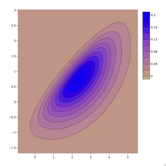
Normale asymétrique bivariée
${\xi}={\begin{pmatrix} 1 \\ 2 \end{pmatrix}},\quad { \Omega }={\begin{pmatrix} 1 & 0.5 \\ 0.5 & 2 \end{pmatrix}}$, ${\alpha}={\begin{pmatrix} -3 \\ 3 \end{pmatrix}}$.

Depuis la bibliothèque sn :
dmsn(x, xi, Omega, alpha)
pmsn(x, xi, Omega, alpha)
rmsn(n, xi, Omega, alpha)
xi, Omega, alphaDepuis la bibliothèque sn :
dmst(x, xi, Omega, alpha, nu)
pmst(x, xi, Omega, alpha, nu)
rmst(n, xi, Omega, alpha, nu )
xi, Omega, alpha, nu (degrés de liberté)Générer 2000 échantillons d'une normale asymétrique en 3D
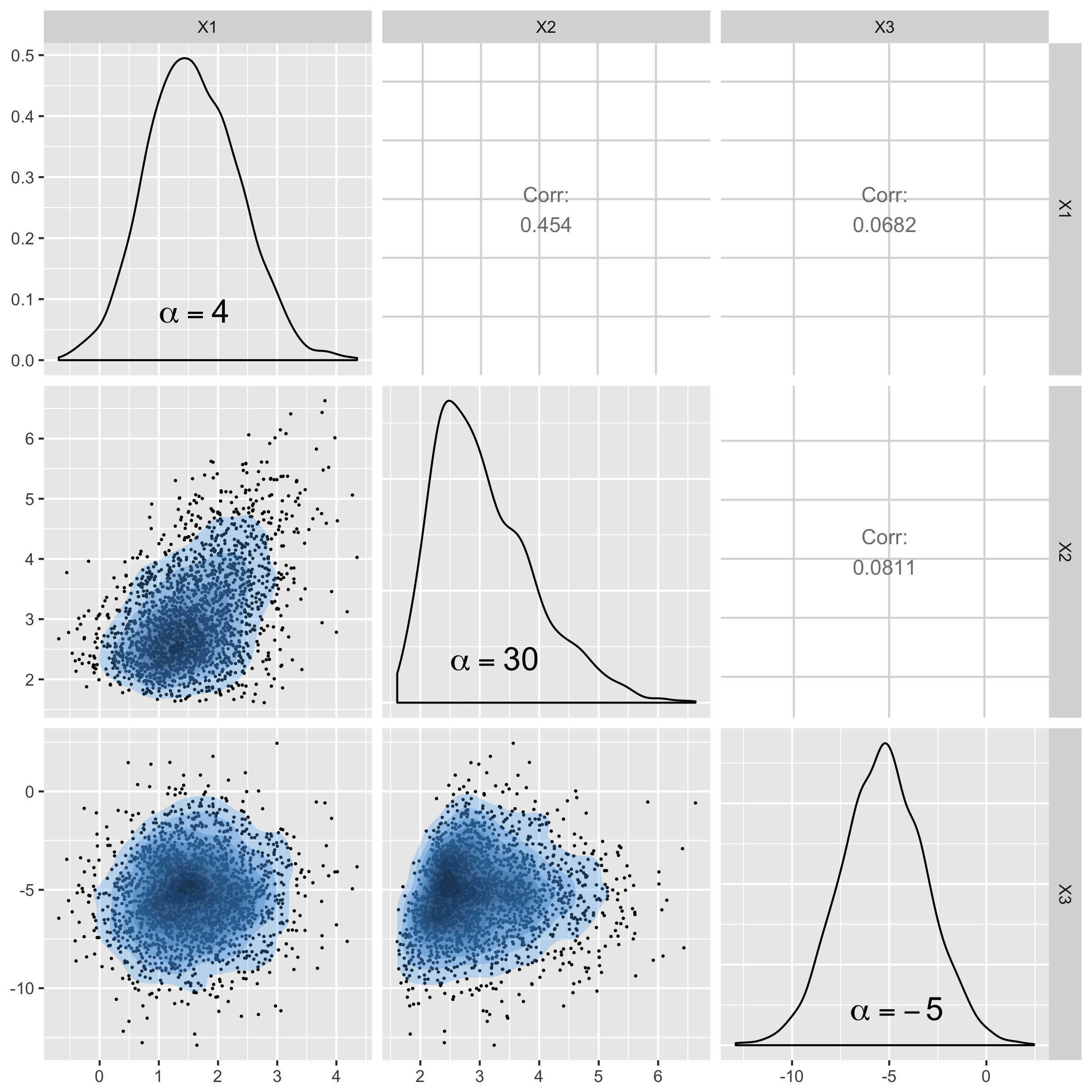
$ SN\left(\xi= \begin{pmatrix} 1 \\ 2 \\ -5 \end{pmatrix} , \Omega={\begin{pmatrix} 1 & 1 & 0 \\ 1 & 2 & 0 \\ 0 & 0 & 5 \end{pmatrix}}, \alpha=\begin{pmatrix} 4 \\ 30 \\ -5 \end{pmatrix} \right)$
# Spécifier xi, Omega et alpha
xi1 <- c(1, 2, -5)
Omega1 <- matrix(c(1, 1, 0,
1, 2, 0,
0, 0, 5), 3, 3)
alpha1 <- c(4, 30, -5)
# Générer des échantillons
skew.sample <- rmsn(n = 2000, xi = xi1, Omega = Omega1, alpha = alpha1)
Échantillon d'une distribution normale asymétrique
Générer 2000 échantillons d'une loi t asymétrique en 3D avec
$\xi= \begin{pmatrix} 1 \\ 2 \\ -5 \end{pmatrix} , \Omega={\begin{pmatrix} 1 & 1 & 0 \\ 1 & 2 & 0 \\ 0 & 0 & 5 \end{pmatrix}}, \alpha=\begin{pmatrix} 4 \\ 30 \\ -5 \end{pmatrix}, df = 4$
# Générer des échantillons
skewt.sample <- rmst(n = 2000, xi = xi1, Omega = Omega1, alpha = alpha1, nu = 4)
Un algorithme itératif est nécessaire pour estimer les paramètres d'une normale asymétrique
Plusieurs fonctions dans le paquet sn, dont msn.mle()
msn.mle(y = skew.sample, opt.method = "BFGS")
$dp
$dp$beta
X1 X2 X3
[1,] 1.024 2.021 -4.81
$dp$Omega
X1 X2 X3
X1 0.9154 0.8865 -0.1507
X2 0.8865 1.8276 -0.3560
X3 -0.1507 -0.3560 5.0352
$dp$alpha
X1 X2 X3
3.670 28.465 -5.029
Les échantillons ont été générés avec :
$\xi= \begin{pmatrix} 1 \\ 2 \\ -5 \end{pmatrix} , \Omega={\begin{pmatrix} 1 & 1 & 0 \\ 1 & 2 & 0 \\ 0 & 0 & 5 \end{pmatrix}}, \alpha=\begin{pmatrix} 4 \\ 30 \\ -5 \end{pmatrix} $
Lois de probabilité multivariée en R