Explaining house price with year & size

Modeling with Data in the Tidyverse

Albert Y. Kim

Assistant Professor of Statistical and Data Sciences

Refresher: Seattle house prices

library(dplyr)
library(moderndive)

# Preview only certain variables:
house_prices %>% 
  select(price, sqft_living, condition, waterfront) %>% 
  glimpse()

Observations: 21,613
Variables: 4
$ price       <dbl> 221900, 538000, 180000, 604000...
$ sqft_living <int> 1180, 2570, 770, 1960, 1680, 5420...
$ condition   <fct> 3, 3, 3, 5, 3, 3, 3, 3, 3, 3, 3...

Refresher: Price and size variables

Refresher: log10 transformation

Refresher: Data transformation

# log10() transform price and size
house_prices <- house_prices %>%
  mutate(
    log10_price = log10(price),
    log10_size = log10(sqft_living)
  )

Model for house price

Outcome variable $y$ - house price (USD): price
Two numerical explanatory/predictor variables:
- $x_1$ - house size: log10_size
- $x_2$ - year built: yr_built

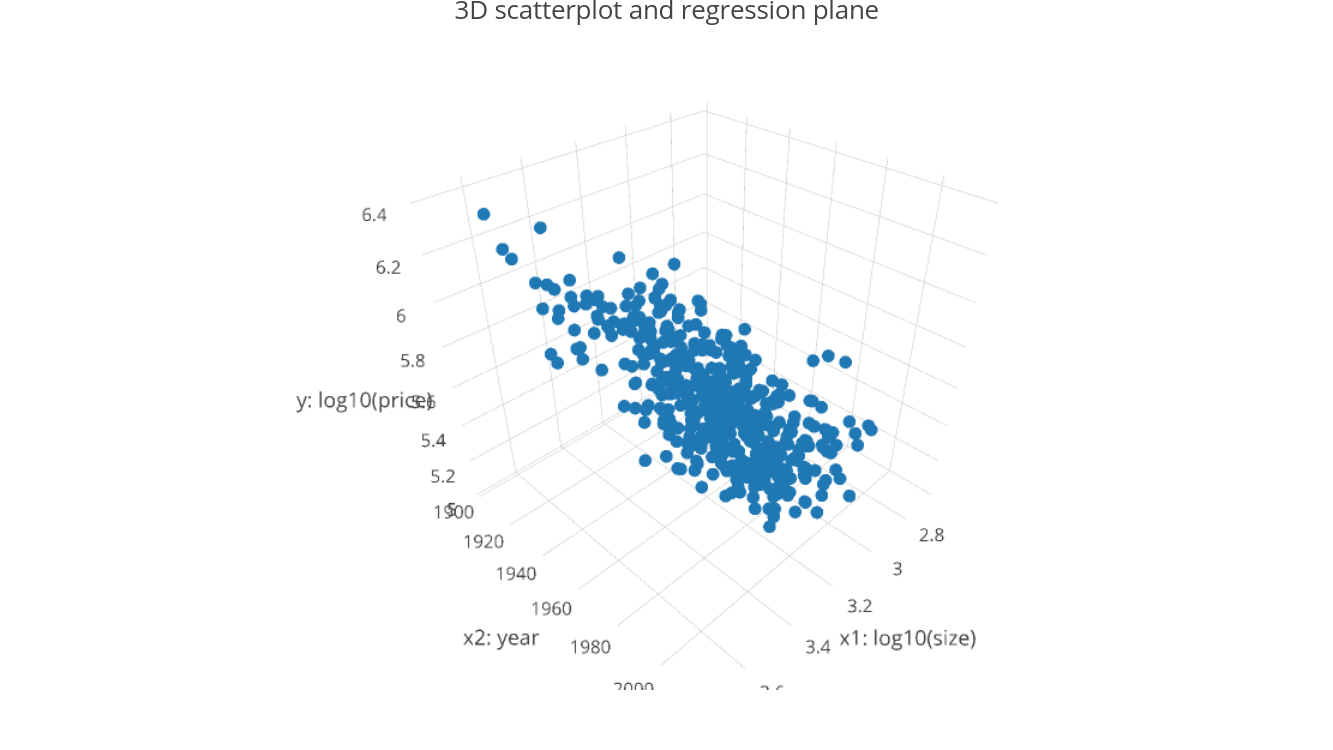
Exploratory visualizing of house price, size & year

3D scatterplot of log10_price, log10_size, and yr_built

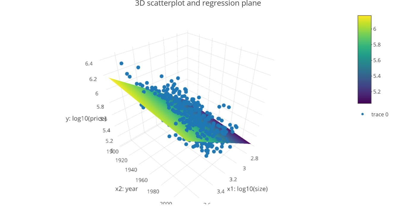
Regression plane

3D scatterplot with regression plane (link to interactive version).

Regression table

# Fit regression model using formula of form: y ~ x1 + x2
model_price_1 <- lm(log10_price ~ log10_size + yr_built, 
                    data = house_prices)

# Output regression table
get_regression_table(model_price_1)

# A tibble: 3 x 7
  term       estimate std_error statistic p_value...
  <chr>         <dbl>     <dbl>     <dbl>   <dbl>...
1 intercept   5.38      0.0754       71.4       0...
2 log10_size  0.913     0.00647     141.        0...
3 yr_built   -0.00138   0.00004     -33.8       0...

Let's practice!

Modeling with Data in the Tidyverse