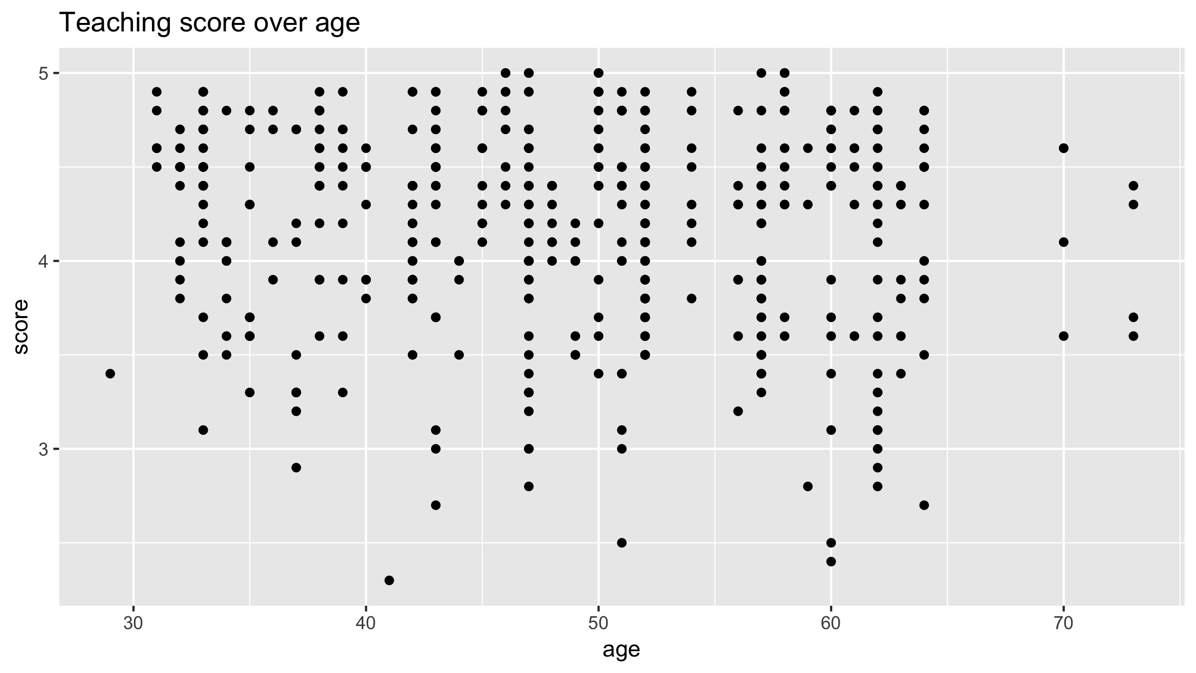
Explaining teaching score with age

Modeling with Data in the Tidyverse

Albert Y. Kim

Assistant Professor of Statistical and Data Sciences

Refresher: Exploratory data visualization

Regression line

# Code to create scatterplot
ggplot(evals, aes(x = age, y = score)) +
  geom_point() + 
  labs(x = "age", y = "score", 
       title = "Teaching score over age")

# Add a "best-fitting" line
ggplot(evals, aes(x = age, y = score)) +
  geom_point() + 
  labs(x = "age", y = "score", 
       title = "Teaching score over age") +
  geom_smooth(method = "lm", se = FALSE)

Regression line

Refresher: Modeling in general

Truth: Assumed model is $y = f(\vec{x}) + \epsilon$
Goal: Given $y$ and $\vec{x}$, fit a model $\hat{f}(\vec{x})$ that approximates $f(\vec{x})$, where $\hat{y} = \hat{f}(\vec{x})$ is the fitted/predicted value for the observed value $y$

Modeling with basic linear regression

Truth:
- Assume $f(x) = \beta_0 + \beta_1 \cdot x$
- Observed value $y = f(x) + \epsilon = \beta_0 + \beta_1 \cdot x + \epsilon$
Fitted:
- Assume $\hat{f}(x) = \hat{\beta}_0 + \hat{\beta}_1 \cdot x$
- Fitted/predicted value $\hat{y} = \hat{f}(x) = \hat{\beta}_0 + \hat{\beta}_1 \cdot x$

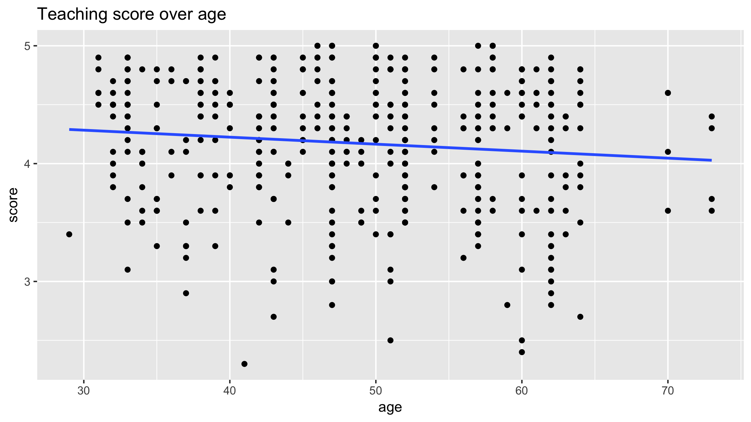
Back to regression line

Equation for fitted blue regression line: $\hat{y} = \hat{f}(\vec{x}) = \hat{\beta}_0 + \hat{\beta}_1 \cdot x$

Computing slope and intercept of regression line

Using the formula form y ~ x:

# Fit regression model using formula of form: y ~ x
model_score_1 <- lm(score ~ age, data = evals)

# Output contents
model_score_1

Call:
lm(formula = score ~ age, data = evals)

Coefficients:
(Intercept)          age  
   4.461932    -0.005938

Computing slope and intercept of regression line

Using the formula form y ~ x, which is akin to $\hat{y}= \hat{f}(\vec{x})$

# Fit regression model using formula of form: y ~ x
model_score_1 <- lm(score ~ age, data = evals)

# Output regression table using wrapper function:
get_regression_table(model_score_1)

# A tibble: 2 x 7
  term      estimate std_error statistic p_value...
  <chr>        <dbl>     <dbl>     <dbl>   <dbl>... 
1 intercept    4.46      0.127     35.2    0...
2 age         -0.006     0.003     -2.31   0.021...

Let's practice!

Modeling with Data in the Tidyverse