The modeling problem for explanation
Modeling with Data in the Tidyverse

Albert Y. Kim
Assistant Professor of Statistical and Data Sciences
Modeling for explanation example
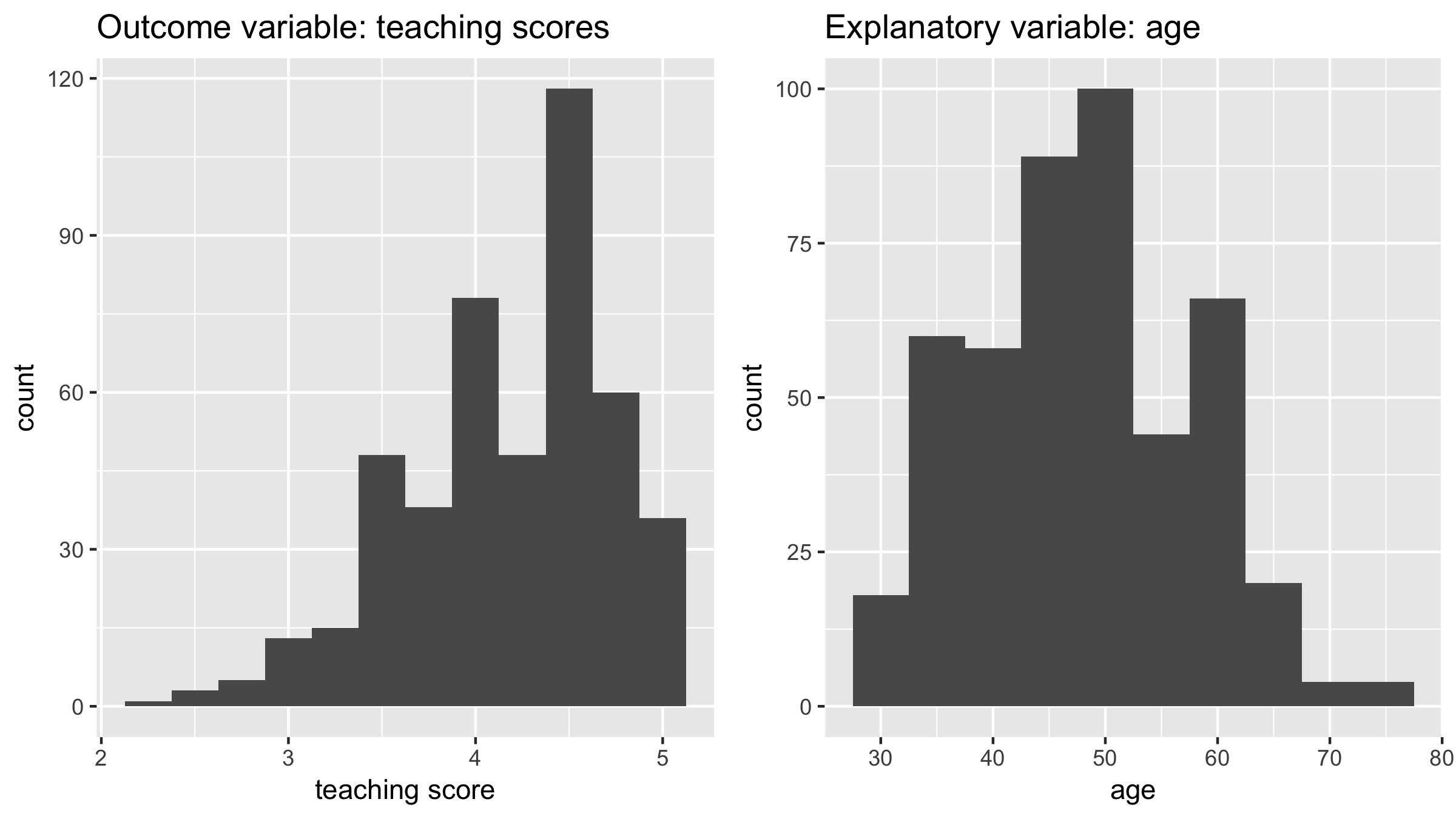
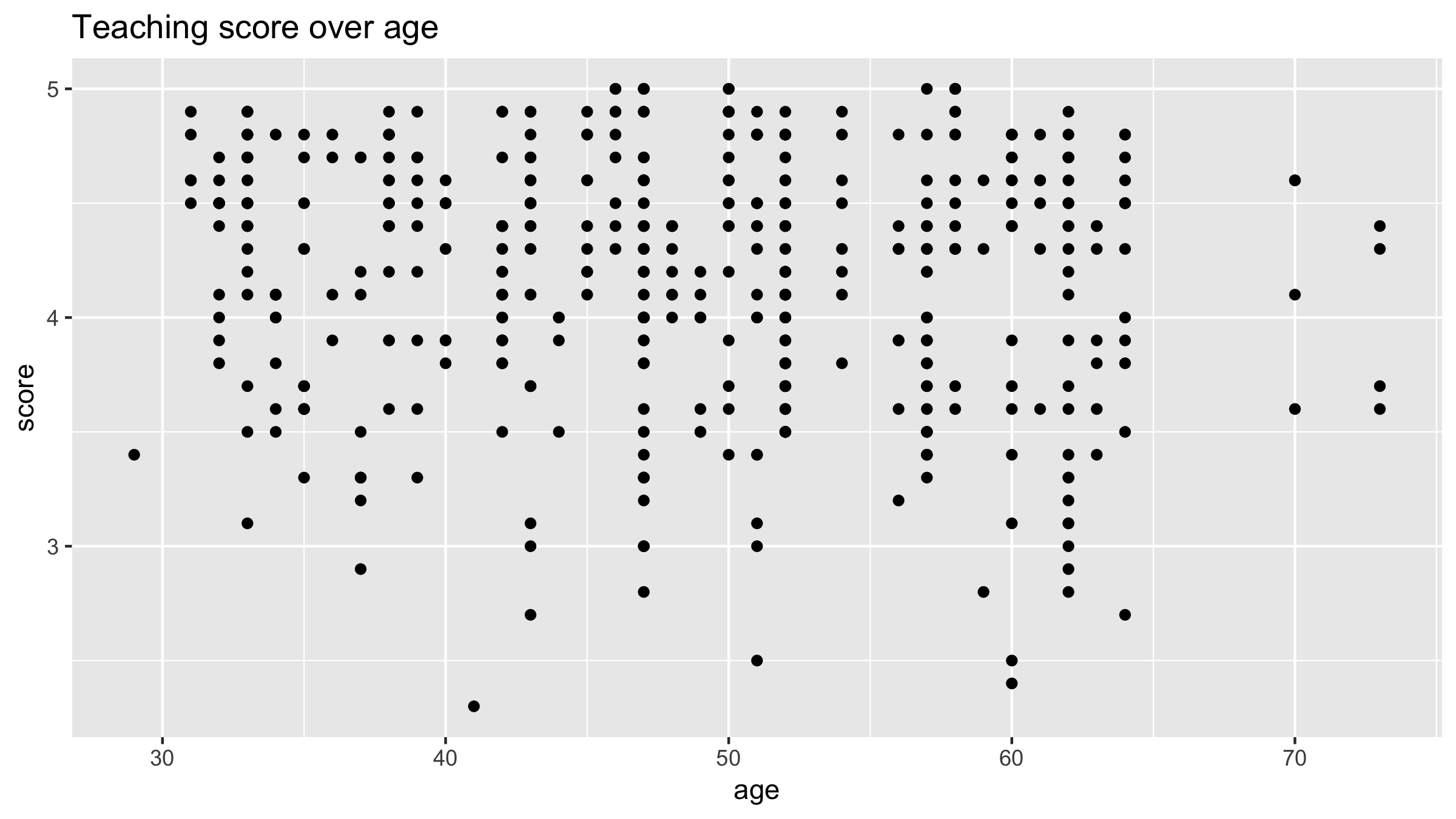
EDA of relationship
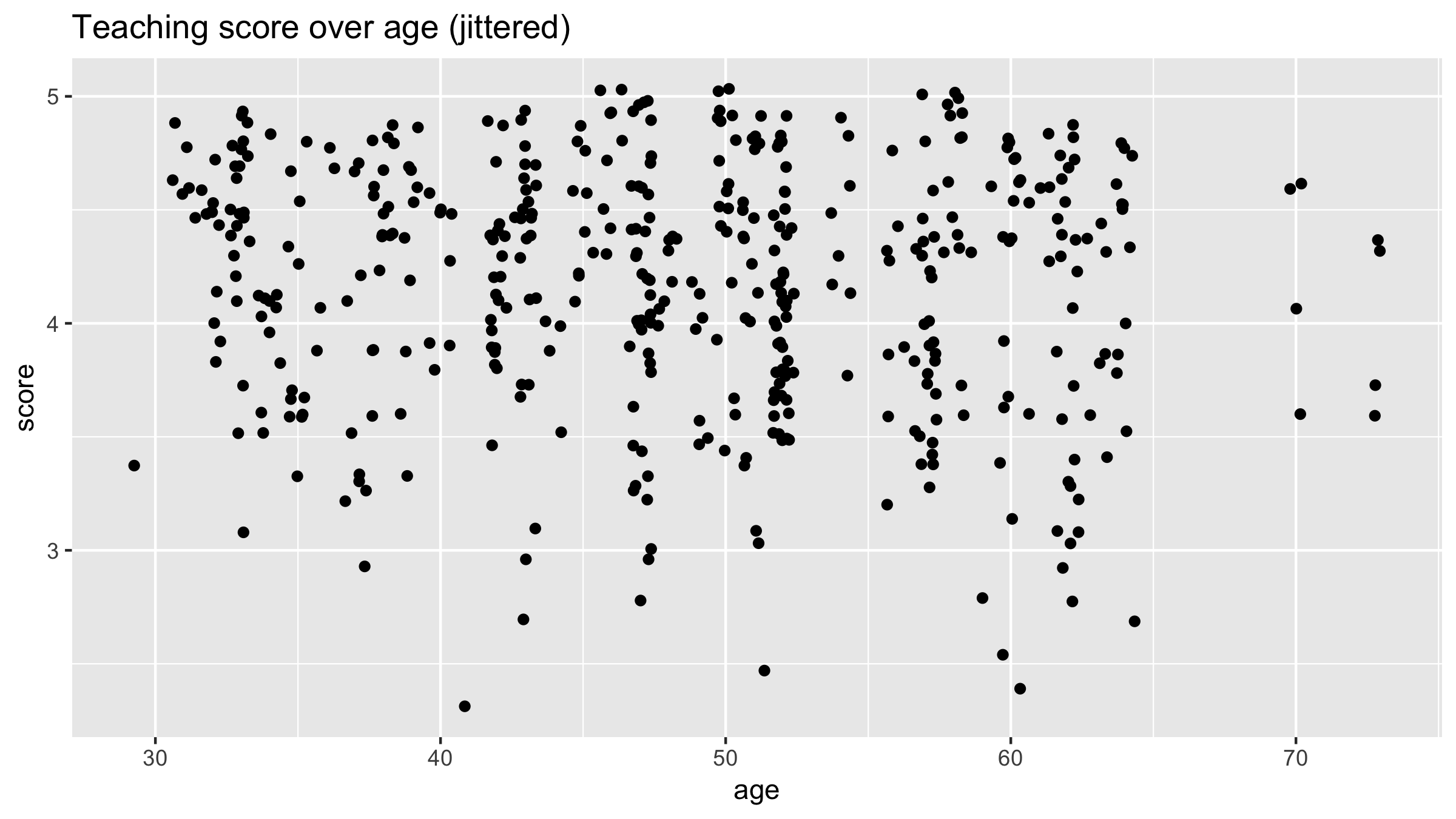
Jittered scatterplot
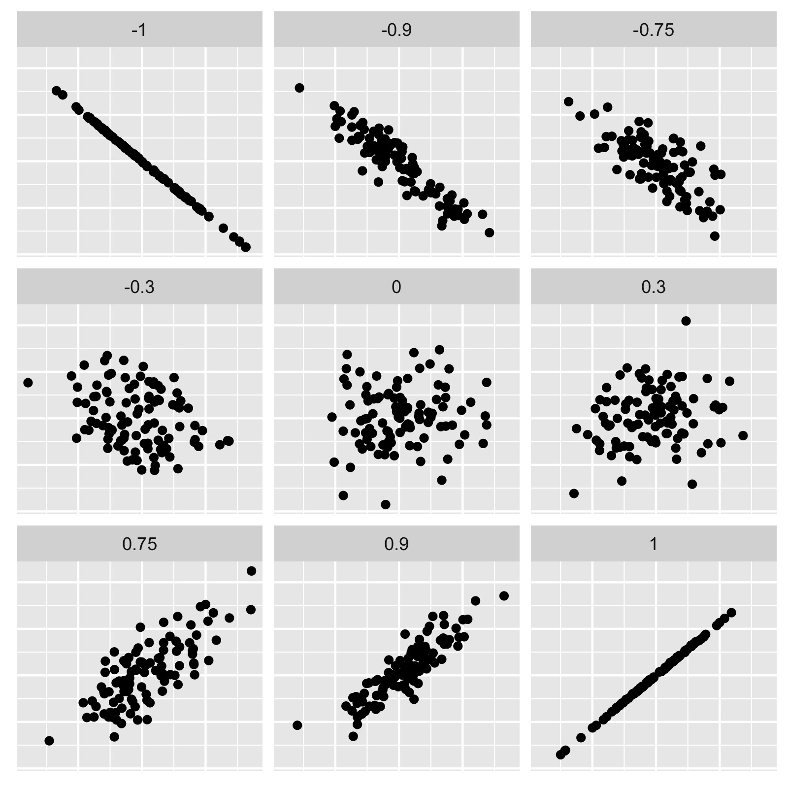
Correlation coefficient
Modeling with Data in the Tidyverse
Albert Y. Kim
Assistant Professor of Statistical and Data Sciences

