Predicting house price using year & size

Modeling with Data in the Tidyverse

Albert Y. Kim

Assistant Professor of Statistical and Data Sciences

Refresher: regression plane

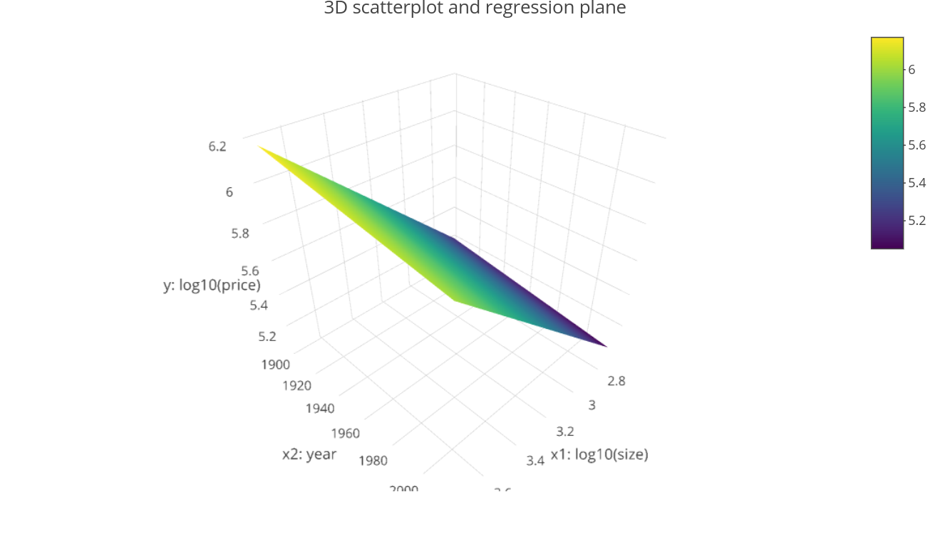
Regression plane for prediction

Predicted value

# Fit regression model using formula of form: y ~ x1 + x2
model_price_1 <- lm(log10_price ~ log10_size + yr_built, 
                    data = house_prices)

# Output regression table
get_regression_table(model_price_1)

# A tibble: 3 x 7
  term       estimate std_error statistic p_value lower_ci...
  <chr>         <dbl>     <dbl>     <dbl>   <dbl>    <dbl>...
1 intercept   5.38      0.0754       71.4       0  5.24...
2 log10_size  0.913     0.00647     141.        0  0.901...
3 yr_built   -0.00138   0.00004     -33.8       0 -0.00146...

Predicted value

# Make prediction
5.38 + 0.913 * 3.07 - 0.00138 * 1980

5.45051

# Convert back to original untransformed units
10^(5.45051)

282169.5

Computing all predicted values and residuals

# Output point-by-point information
get_regression_points(model_price_1)

# A tibble: 21,613 x 6
      ID log10_price log10_size yr_built log10_price_hat
   <int>       <dbl>      <dbl>    <dbl>           <dbl>
 1     1        5.35       3.07     1955            5.50
 2     2        5.73       3.41     1951            5.81
 3     3        5.26       2.89     1933            5.36
 4     4        5.78       3.29     1965            5.69
 5     5        5.71       3.22     1987            5.60
 6     6        6.09       3.73     2001            6.04
 7     7        5.41       3.23     1995            5.59
...

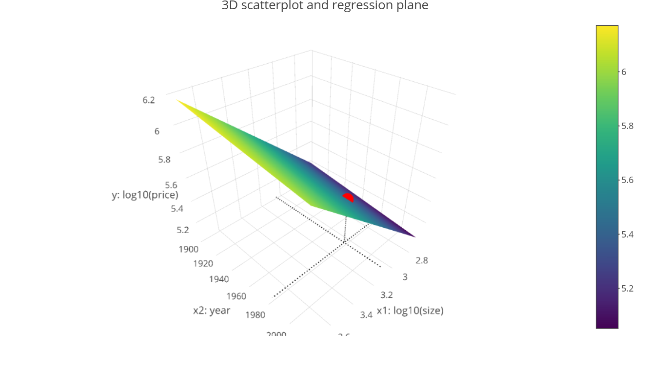
Best fit and residuals

Sum of squared residuals

# A tibble: 21,613 x 6
      ID log10_price log10_size yr_built log10_price_hat
   <int>       <dbl>      <dbl>    <dbl>           <dbl>
 1     1        5.35       3.07     1955            5.50
 2     2        5.73       3.41     1951            5.81
...

# Square all residuals and sum them
get_regression_points(model_price_1) %>%
  mutate(sq_residuals = residual^2) %>%
  summarize(sum_sq_residuals = sum(sq_residuals))

# A tibble: 1 x 1
  sum_sq_residuals
             <dbl>
1             585.

Let's practice!

Modeling with Data in the Tidyverse