स्पेक्ट्रोग्राम - समय के साथ ध्वनि में स्पेक्ट्रल बदलाव

Python में Time Series Data के लिए Machine Learning

Chris Holdgraf

Fellow, Berkeley Institute for Data Science

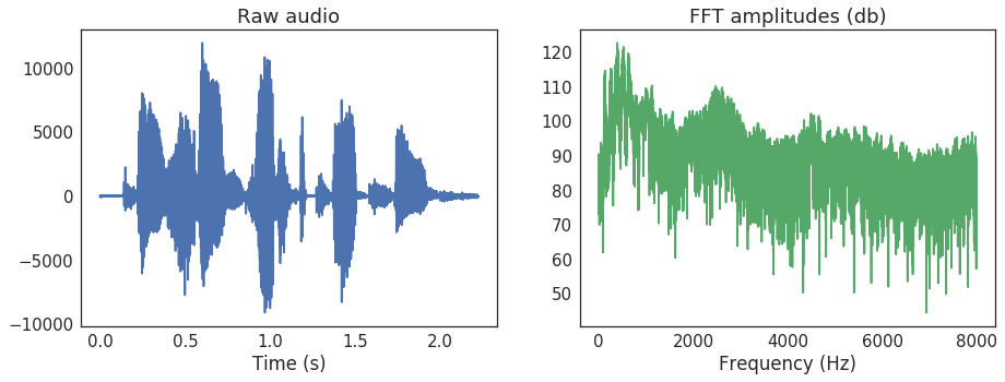
Fourier transforms

टाइमसीरीज़ डेटा को तेज़ी से बदलने वाली और धीरे-धीरे बदलने वाली चीज़ों के संयोजन के रूप में वर्णित किया जा सकता है
हर समय-बिंदु पर, तेज़ और धीमे घटकों की सापेक्ष उपस्थिति बताई जा सकती है
इसे करने का सबसे सरल तरीका Fourier Transform है
यह एक टाइमसीरीज़ को दोलनों के संयोजन के रूप में बताने वाली एक array में बदल देता है

एक Fourier Transform (FFT)

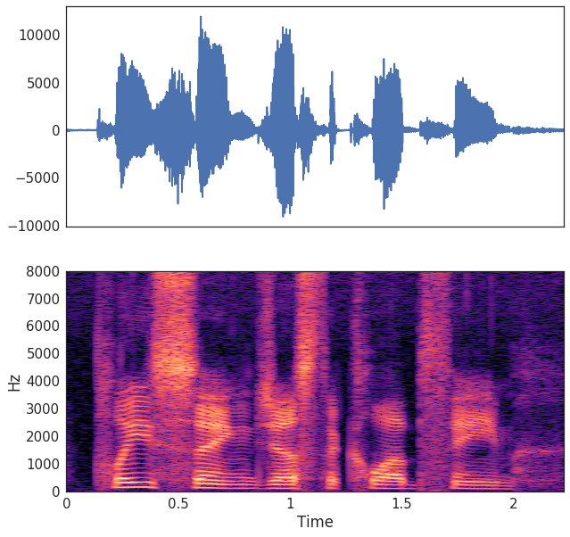
स्पेक्ट्रोग्राम: विंडो वाले Fourier transforms का संयोजन

स्पेक्ट्रोग्राम समय के साथ विंडो किए गए Fourier transforms का संग्रह होता है
जैसे रोलिंग मीन निकाला था:
1. विंडो का आकार और आकार चुनें
2. किसी समय-बिंदु पर उस विंडो की FFT निकालें
3. विंडो को एक स्टेप सरकाएँ
4. परिणाम समेकित करें
इसे Short-Time Fourier Transform (STFT) कहते हैं

STFT की गणना

हम librosa से STFT निकाल सकते हैं
कई पैरामीटर ट्यून किए जा सकते हैं (जैसे विंडो साइज)
हमारे काम के लिए, हम इसे decibels में बदलेंगे, जो सभी फ़्रीक्वेंसी के औसत मानों को normalizes करता है
फिर specshow() फंक्शन से इसे विज़ुअलाइज़ करेंगे

कोड से STFT निकालना

# Import the functions we'll use for the STFT
from librosa.core import stft, amplitude_to_db
from librosa.display import specshow
import matplotlib.pyplot as plt

# Calculate our STFT
HOP_LENGTH = 2**4
SIZE_WINDOW = 2**7
audio_spec = stft(audio, hop_length=HOP_LENGTH, n_fft=SIZE_WINDOW)

# Convert into decibels for visualization
spec_db = amplitude_to_db(audio_spec)

# Visualize
fig, ax = plt.subplots()
specshow(spec_db, sr=sfreq, x_axis='time', 
         y_axis='hz', hop_length=HOP_LENGTH, ax=ax)

स्पेक्ट्रल फीचर इंजीनियरिंग

हर टाइमसीरीज़ का अलग स्पेक्ट्रल पैटर्न होता है.
हम स्पेक्ट्रोग्राम का विश्लेषण करके ये पैटर्न निकाल सकते हैं.
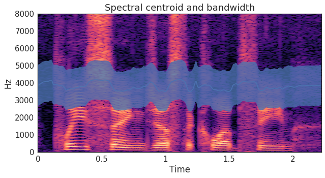
जैसे, spectral bandwidth और spectral centroids बताते हैं कि हर पल अधिकतर ऊर्जा कहाँ है

स्पेक्ट्रल फीचर्स की गणना

# Calculate the spectral centroid and bandwidth for the spectrogram
bandwidths = lr.feature.spectral_bandwidth(S=spec)[0]
centroids = lr.feature.spectral_centroid(S=spec)[0]

# Display these features on top of the spectrogram
fig, ax = plt.subplots()
specshow(spec, x_axis='time', y_axis='hz', hop_length=HOP_LENGTH, ax=ax)
ax.plot(times_spec, centroids)
ax.fill_between(times_spec, centroids - bandwidths / 2, 
                centroids + bandwidths / 2, alpha=0.5)

क्लासिफायर में स्पेक्ट्रल और टेम्पोरल फीचर्स मिलाना

centroids_all = []
bandwidths_all = []
for spec in spectrograms:
    bandwidths = lr.feature.spectral_bandwidth(S=lr.db_to_amplitude(spec))
    centroids = lr.feature.spectral_centroid(S=lr.db_to_amplitude(spec))
    # Calculate the mean spectral bandwidth
    bandwidths_all.append(np.mean(bandwidths))  
    # Calculate the mean spectral centroid
    centroids_all.append(np.mean(centroids))  

# Create our X matrix
X = np.column_stack([means, stds, maxs, tempo_mean, 
                     tempo_max, tempo_std, bandwidths_all, centroids_all])

अभ्यास करते हैं!

Python में Time Series Data के लिए Machine Learning