विश्वास अंतराल की व्याख्या

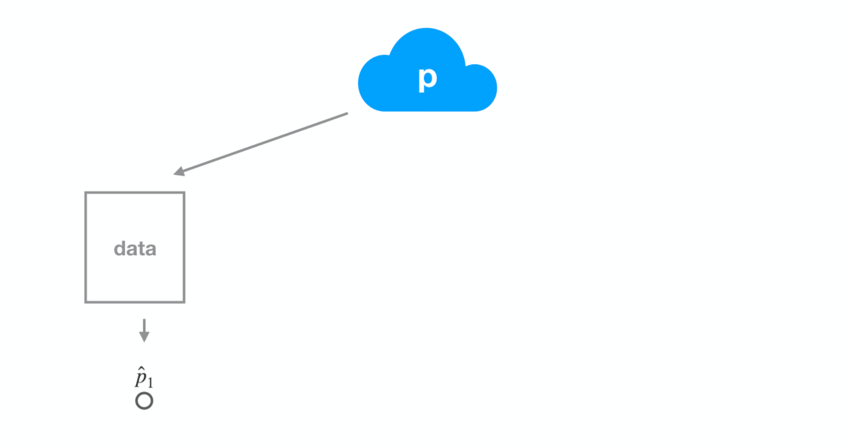
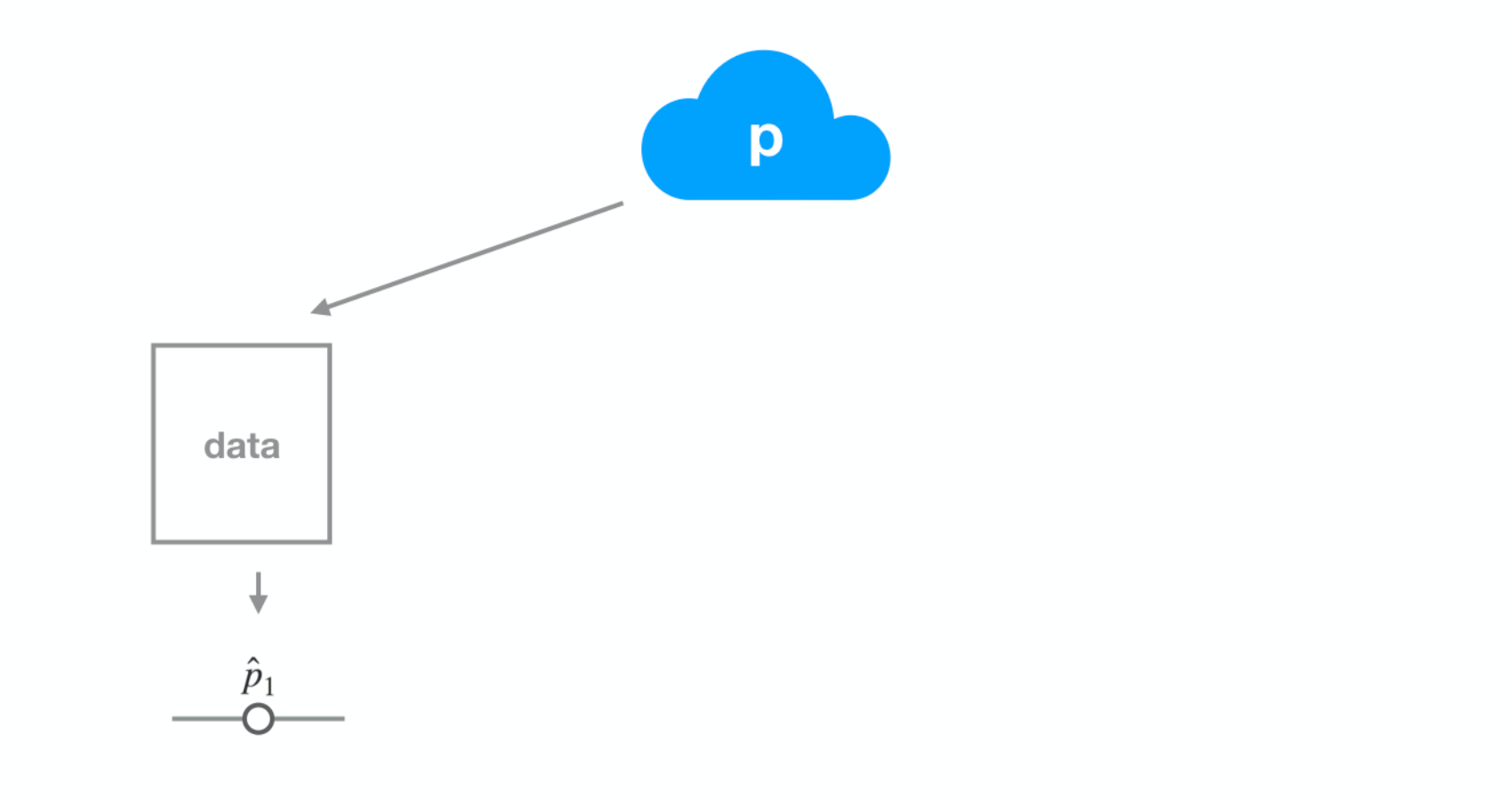
R में श्रेणीबद्ध डेटा के लिए अनुमान

Andrew Bray

Assistant Professor of Statistics at Reed College

Confidence intervals

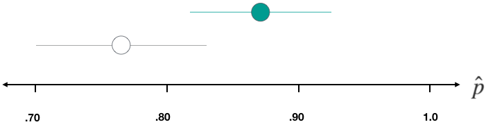
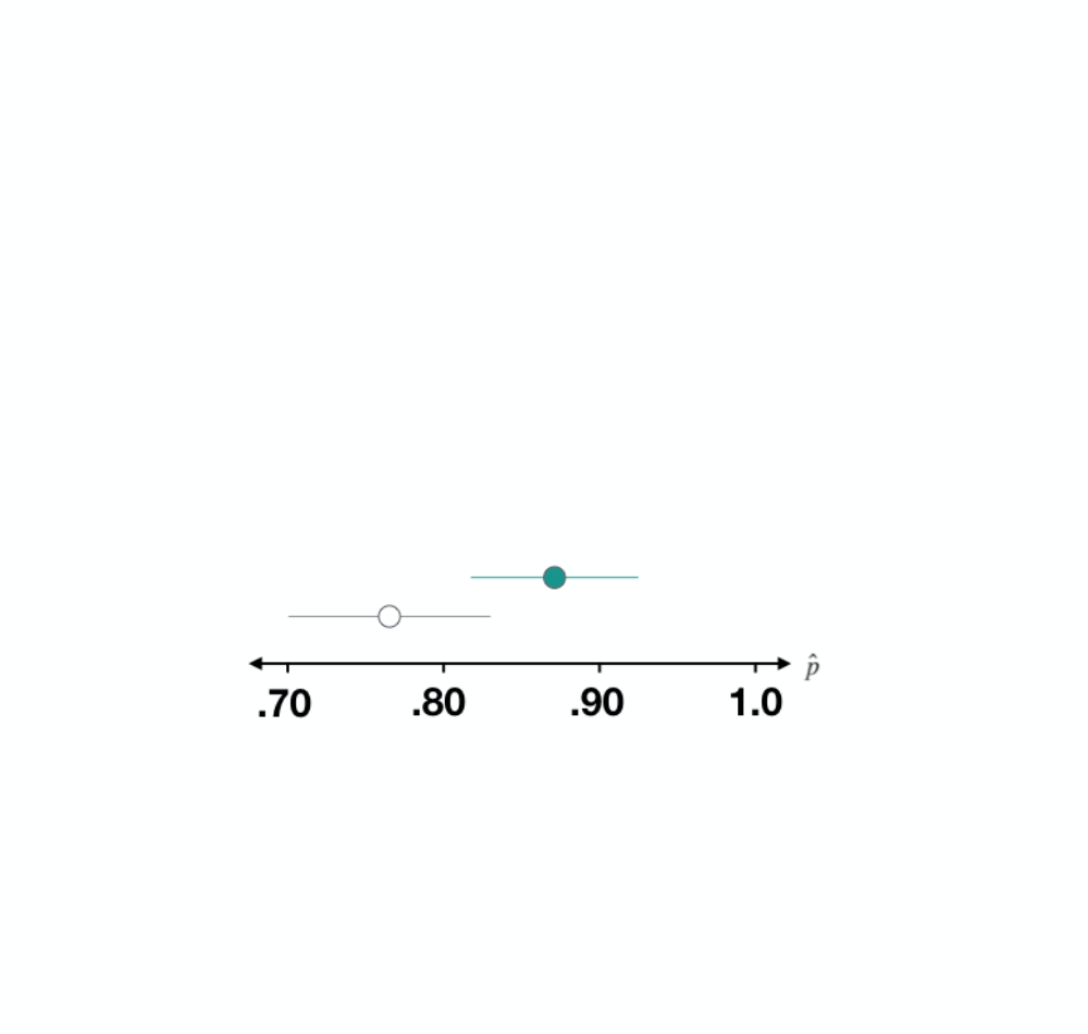
निष्कर्ष: खुश अमेरिकियों का वास्तविक अनुपात 0.705 और 0.841 के बीच है।

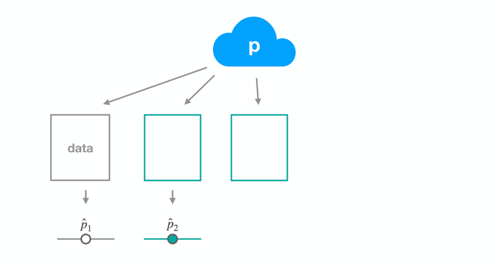
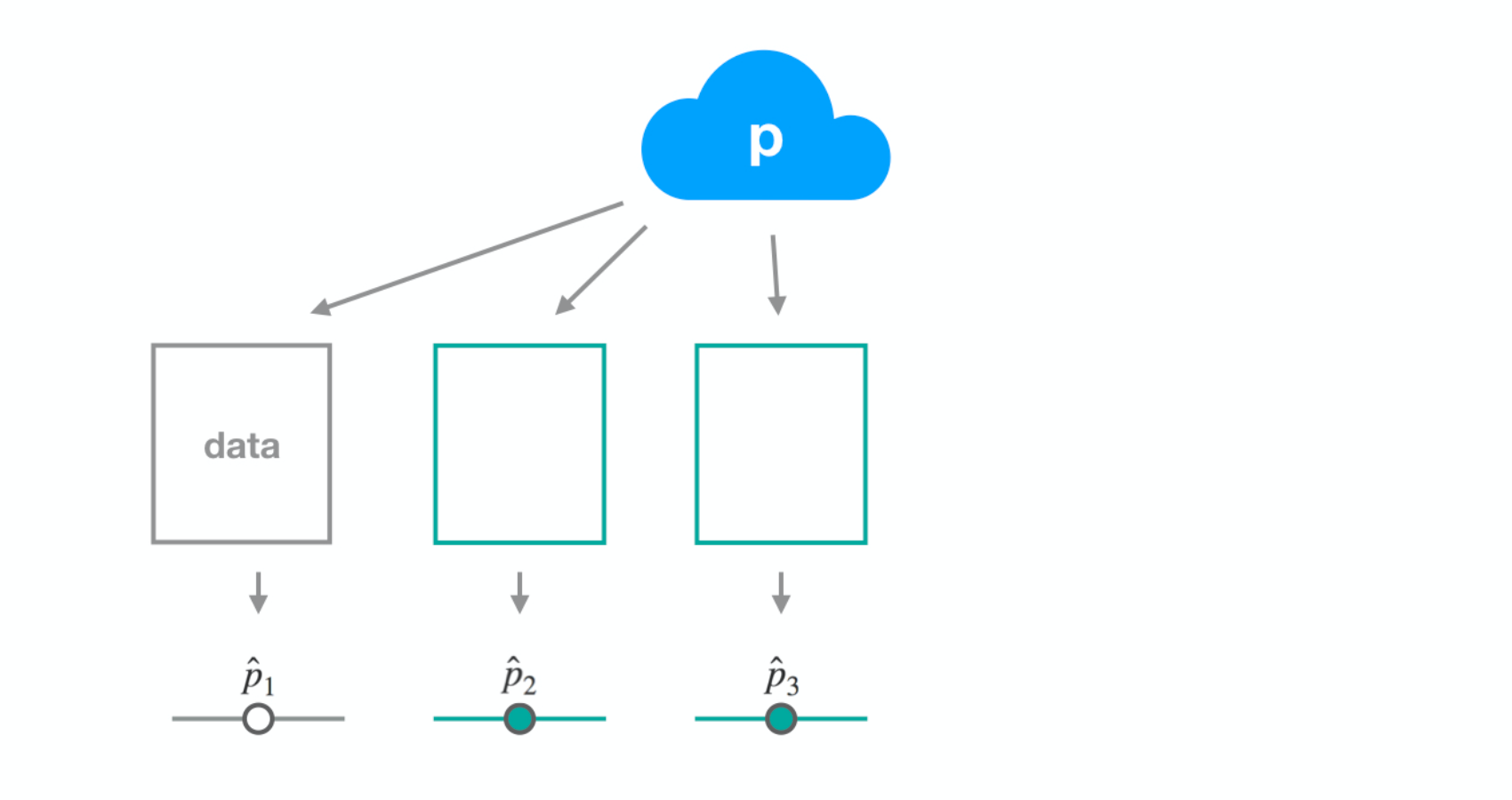
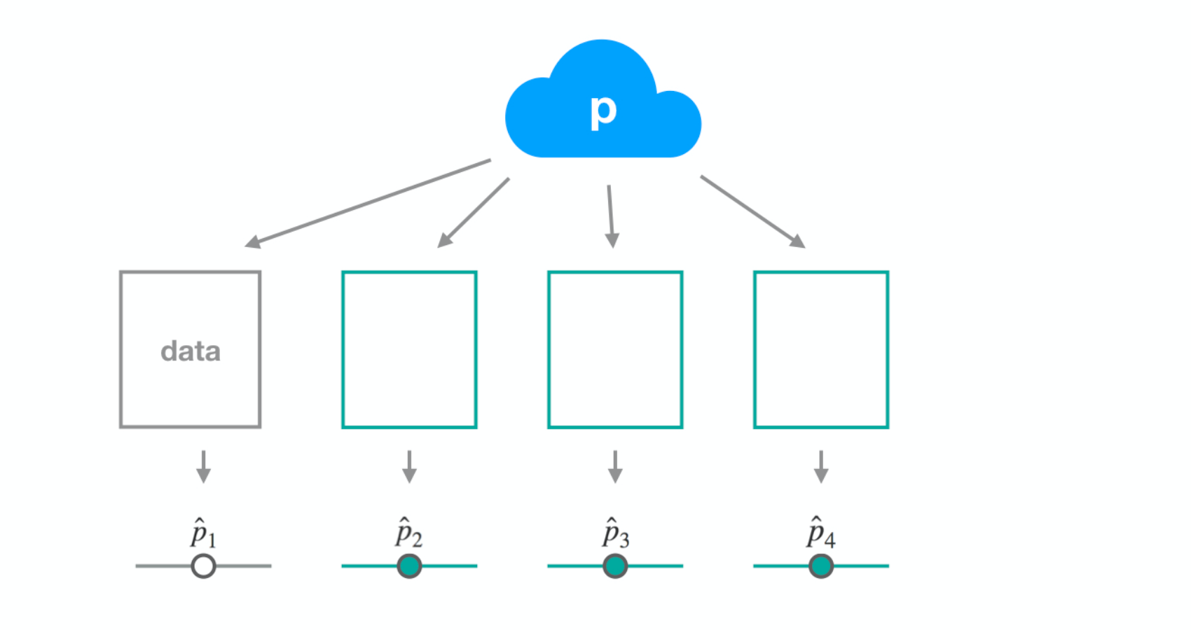
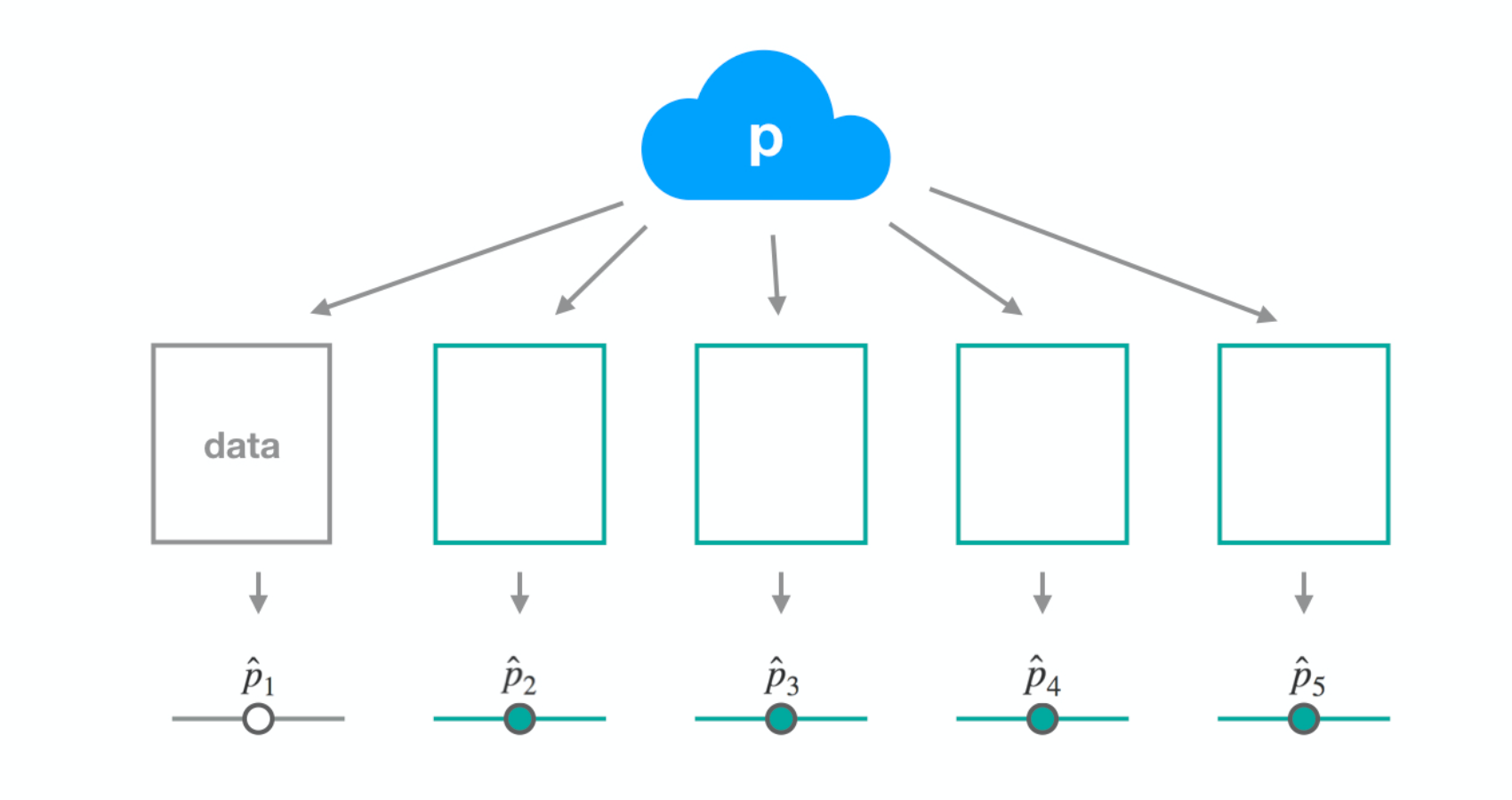
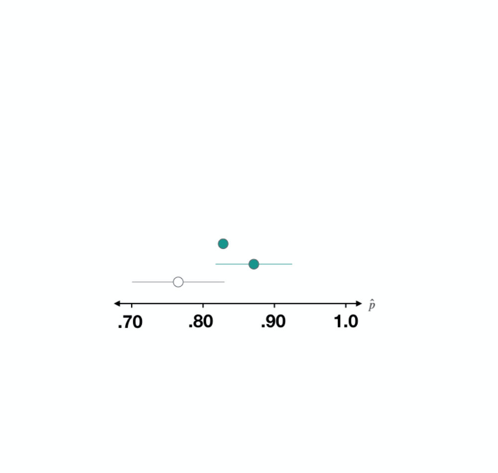
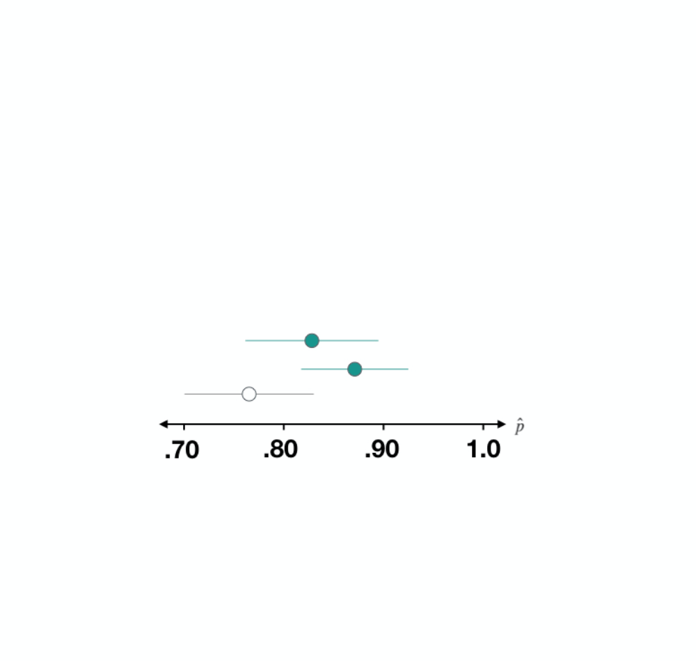
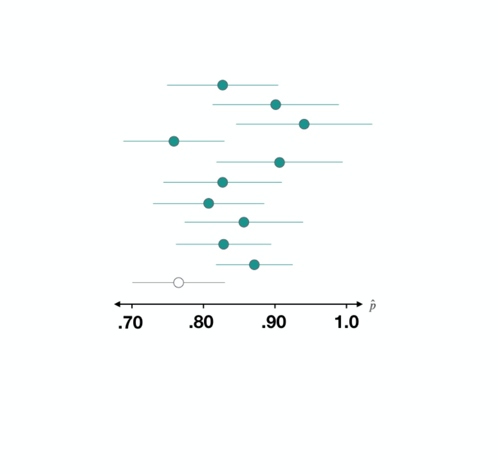
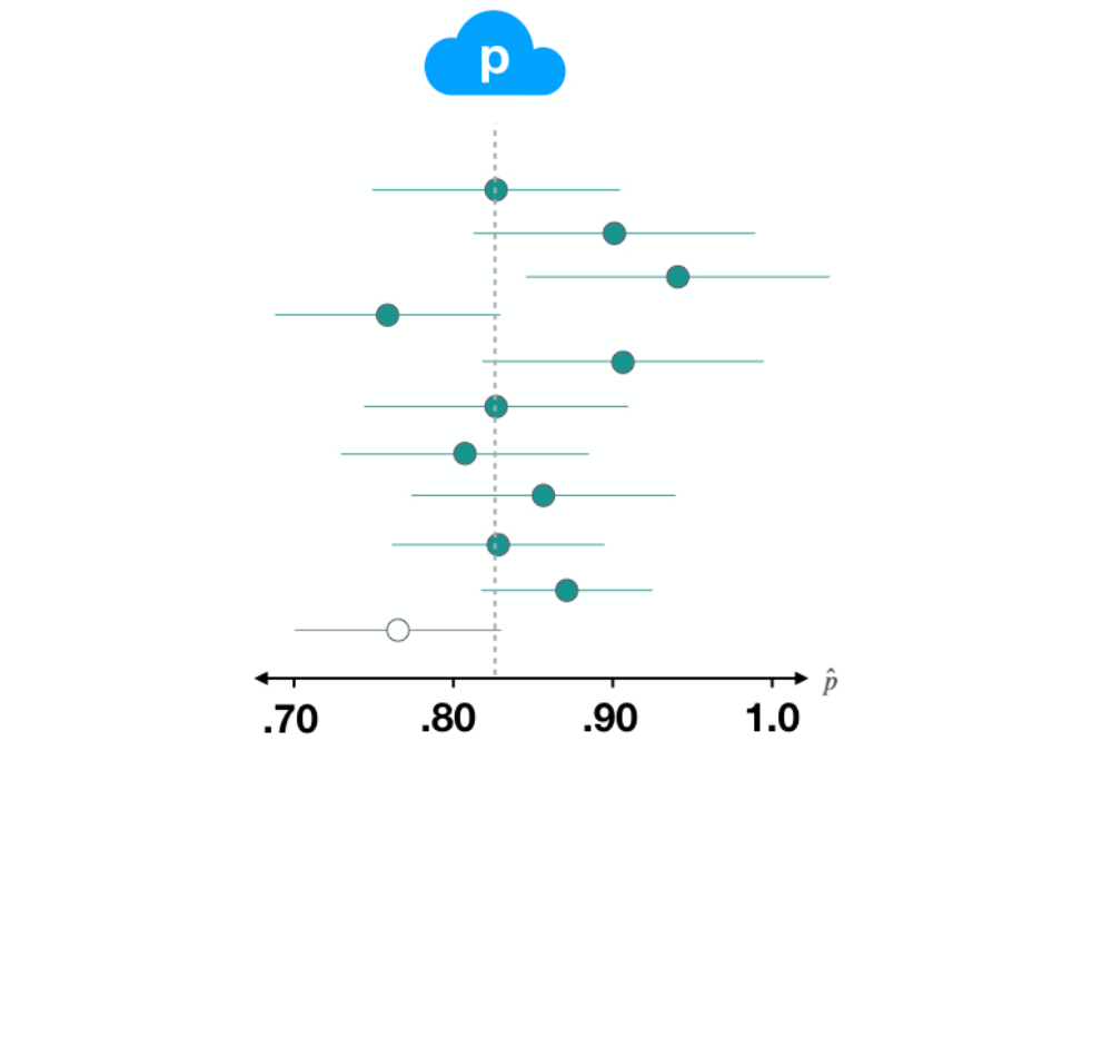
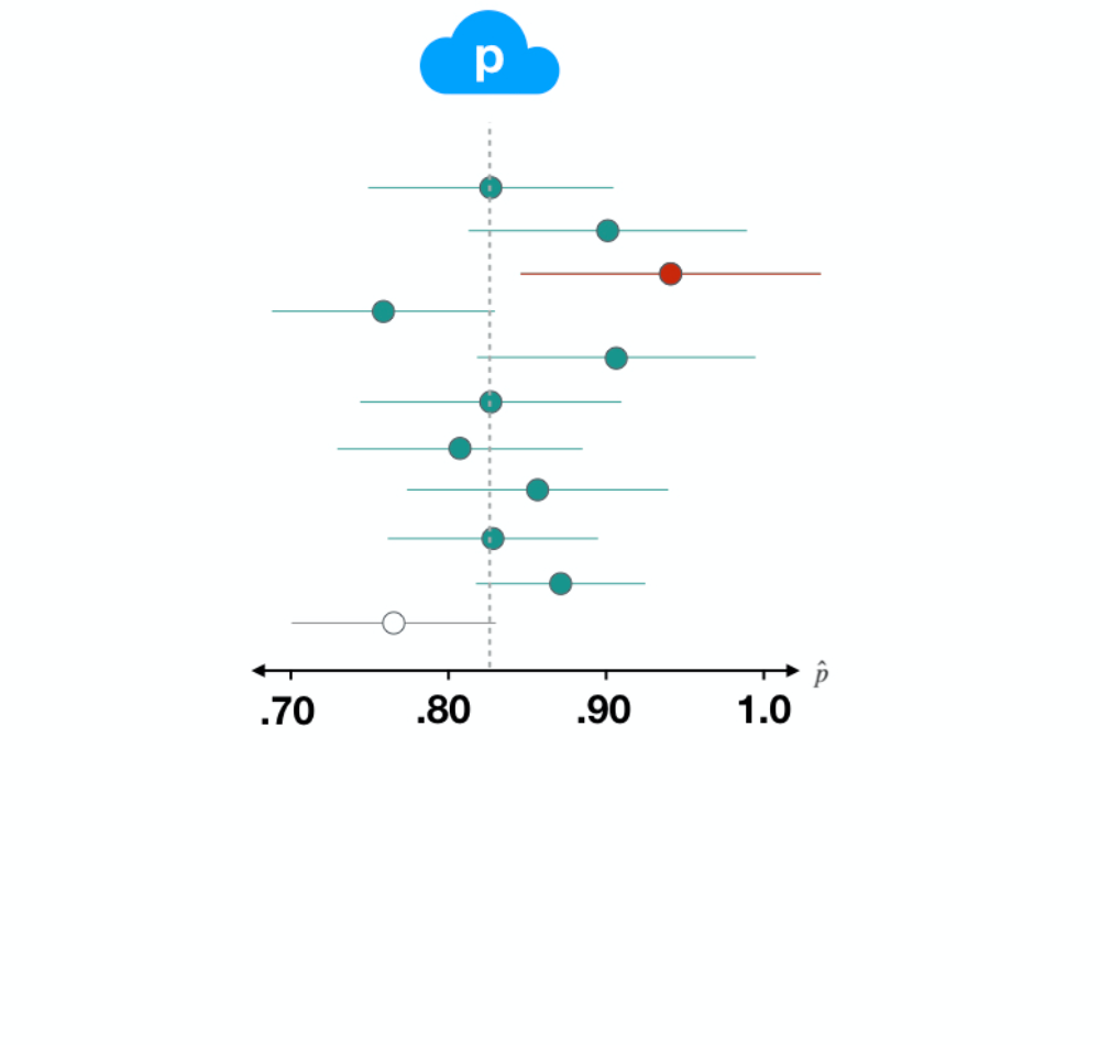
हम "confident" से क्या मतलब लेते हैं?

डेटासेट 1

ds1 <- filter(gss, year == 2016)

p_hat <- ds1 %>%
  summarize(mean(happy == "HAPPY")) %>% 
  pull()

SE <- ds1 %>%
  specify(response = happy, 
          success = "HAPPY") %>%
  generate(reps = 500, 
           type = "bootstrap") %>%
  calculate(stat = "prop") %>%
  summarize(sd(stat)) %>% 
  pull()

c(p_hat - 2 * SE, p_hat + 2 * SE)

0.7073114 0.8393553

विश्वास-अंतराल

डेटासेट 2

ds2 <- filter(gss, year == 2014)

p_hat <- ds1 %>%
  summarize(mean(happy == "HAPPY")) %>% 
  pull()

SE <- ds1 %>%
  specify(response = happy, 
          success = "HAPPY") %>%
  generate(reps = 500, 
           type = "bootstrap") %>%
  calculate(stat = "prop") %>%
  summarize(sd(stat)) %>% 
  pull()

c(p_hat - 2 * SE, p_hat + 2 * SE)

0.8348831 0.9384503

Screenshot 2019-02-21 18.05.03.png

डेटासेट 3

ds3 <- filter(gss, year == 2012)

p_hat <- ds1 %>%
  summarize(mean(happy == "HAPPY")) %>% 
  pull()

SE <- ds1 %>%
  specify(response = happy, 
          success = "HAPPY") %>%
  generate(reps = 500, 
           type = "bootstrap") %>%
  calculate(stat = "prop") %>%
  summarize(sd(stat)) %>% 
  pull()

c(p_hat - 2 * SE, p_hat + 2 * SE)

0.7626359 0.8906974

डेटासेट 3

ds3 <- filter(gss, year == 2012)
p_hat <- ds3 %>%
  summarize(mean(happy == "HAPPY")) %>%
  pull()
SE <- ds3 %>%
  specify(response = happy, 
          success = "HAPPY") %>%
  generate(reps = 500, 
           type = "bootstrap") %>%
  calculate(stat = "prop") %>%
  summarize(sd(stat)) %>%
  pull()

c(p_hat - 2 * SE, p_hat + 2 * SE)

0.7626359 0.8906974

डेटासेट 3

ds3 <- filter(gss, year == 2012)
p_hat <- ds3 %>%
  summarize(mean(happy == "HAPPY")) %>%
  pull()
SE <- ds3 %>%
  specify(response = happy, 
          success = "HAPPY") %>%
  generate(reps = 500, 
           type = "bootstrap") %>%
  calculate(stat = "prop") %>%
  summarize(sd(stat)) %>%
  pull()

c(p_hat - 2 * SE, p_hat + 2 * SE)

0.7626359 0.8906974

डेटासेट 3

ds3 <- filter(gss, year == 2012)
p_hat <- ds3 %>%
  summarize(mean(happy == "HAPPY")) %>%
  pull()
SE <- ds3 %>%
  specify(response = happy, 
          success = "HAPPY") %>%
  generate(reps = 500, 
           type = "bootstrap") %>%
  calculate(stat = "prop") %>%
  summarize(sd(stat)) %>%
  pull()

c(p_hat - 2 * SE, p_hat + 2 * SE)

0.7626359 0.8906974

डेटासेट 3

ds3 <- filter(gss, year == 2012)
p_hat <- ds3 %>%
  summarize(mean(happy == "HAPPY")) %>%
  pull()
SE <- ds3 %>%
  specify(response = happy, 
          success = "HAPPY") %>%
  generate(reps = 500, 
           type = "bootstrap") %>%
  calculate(stat = "prop") %>%
  summarize(sd(stat)) %>%
  pull()

c(p_hat - 2 * SE, p_hat + 2 * SE)

0.7626359 0.8906974

डेटासेट 3

ds3 <- filter(gss, year == 2012)
p_hat <- ds3 %>%
  summarize(mean(happy == "HAPPY")) %>%
  pull()
SE <- ds3 %>%
  specify(response = happy, 
          success = "HAPPY") %>%
  generate(reps = 500, 
           type = "bootstrap") %>%
  calculate(stat = "prop") %>%
  summarize(sd(stat)) %>%
  pull()

c(p_hat - 2 * SE, p_hat + 2 * SE)

0.7626359 0.8906974

Confidence Intervals

व्याख्या: "हम 95% confident हैं कि खुश अमेरिकियों का वास्तविक अनुपात 0.705 और 0.841 के बीच है।"

अंतराल की चौड़ाई प्रभावित होती है

n
confidence level
p

अभ्यास करते हैं!

R में श्रेणीबद्ध डेटा के लिए अनुमान