sf के साथ जियोस्पैशियल मैप्स

shinydashboard के साथ डैशबोर्ड बनाना

Png Kee Seng

Researcher

sf का परिचय

जियोस्पैशियल मैप बनाने के लिए sf का उपयोग करें
- "simple features" का संक्षेप
sf विज़ुअलाइज़ेशन हमेशा लेयर्स में बनता है
- जैसे खाली कैनवास पर निपुण ब्रश स्ट्रोक्स की परतें
- हम जियोस्पैशियल विज़ुअलाइज़ेशन में गहराई से नहीं जाएँगे

खाली कैनवास पर ब्रश स्ट्रोक्स.

¹ Image by rawpixel.com on Freepik

लाइब्रेरी और जियोस्पैशियल डेटा इम्पोर्ट करना

sf और tidyverse इम्पोर्ट करें
keyhole markup language (KML) फाइलें पढ़ने के लिए st_read() और st_as_sf() का उपयोग करें
- london_poly: लंदन की जियोस्पैशियल सीमाएँ
- london_loop: लंदन के चारों ओर लगभग गोल _पथ_
- london_capital: इनर लंदन के हिस्सों को जोड़ने वाला गोल _पथ_
- listings_geo: Airbnb लिस्टिंग्स के coordinates

library(sf)
library(tidyverse)

london_poly <- st_read("../data/london_boroughs_boroughs_kml.kml",
                            drivers = "KML", quiet=TRUE)

london_loop <- st_read("../data/London-Loop-SWC-Walk-L24.kml",
                       drivers = "KML", quiet=TRUE)

london_capital <- st_read("../data/Capital-Ring-SWC-Walk-L23.kml",
                          drivers="KML", quiet=TRUE)

listings_geo <- st_as_sf(listings,
                         coords = c("longitude", "latitude"))

sf ऑब्जेक्ट्स के प्रकार: MULTIPOLYGON

london_poly$geometry

Geometry set for 33 features 
Geometry type: MULTIPOLYGON

Dimension:     XY
Bounding box:  xmin: -0.508813 ymin: 51.28691 ...
Geodetic CRS:  WGS 84
First 5 geometries:
MULTIPOLYGON (((-0.183361 51.66868, -0.183383 5...
MULTIPOLYGON (((0.158044 51.50904, 0.156309 51....
MULTIPOLYGON (((-0.212138 51.55558, -0.212689 5...
MULTIPOLYGON (((0.076463 51.431, 0.075932 51.43...
MULTIPOLYGON (((-0.140804 51.56946, -0.14081 51...

10 किनारों वाला रैंडम बहुभुज.

15 किनारों वाला रैंडम बहुभुज.

sf ऑब्जेक्ट्स के प्रकार: LINESTRING

london_loop$geometry

Geometry set for 1 feature 
Geometry type: LINESTRING
Dimension:     XYZ
Bounding box:  xmin: -0.499406 ymin: 51.29375 xmax: 0.257656 ymax: 51.67563
z_range:       zmin: 0 zmax: 174
Geodetic CRS:  WGS 84
LINESTRING Z (0.236477 51.48095 1, 0.235149 51....

london_capital के लिए भी वही

sf ऑब्जेक्ट्स के प्रकार: POINT

listings_geo$geometry

Geometry set for 69351 features 
Geometry type: POINT
Dimension:     XY
Bounding box:  xmin: -0.5236 ymin: 51.27248 xmax: 0.30515 ymax: 51.70893
CRS:           NA
First 5 geometries:
POINT (-0.05396 51.52874)
POINT (-0.1127 51.56861)
POINT (-0.07426 51.52851)
POINT (-0.10484 51.52478)
POINT (-0.20004 51.51464)

plot() से पॉलीगॉन प्लॉट करना

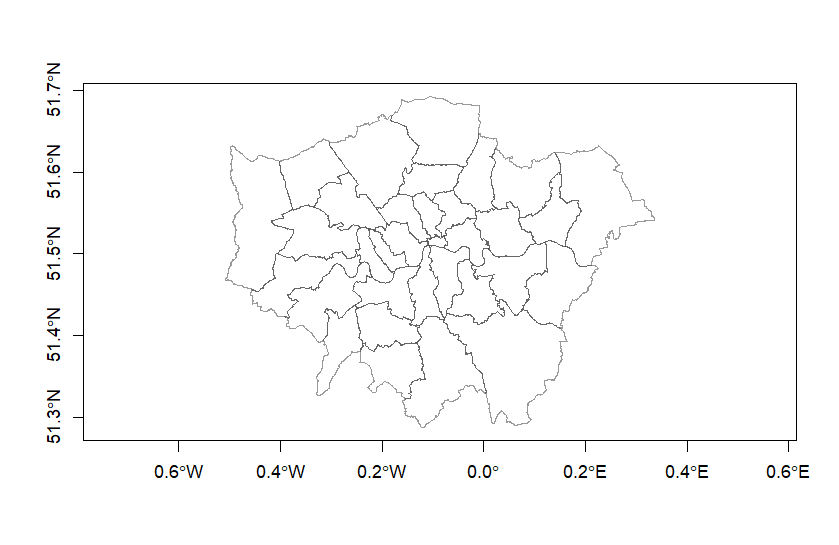
पॉलीगॉन बनाने के लिए st_geometry() का उपयोग करें
plot() का उपयोग करें
अलग रंग भरने के लिए col सेट करें

plot(st_geometry(london_poly), axes=TRUE, 
                border=grey(0.2, 0.5))

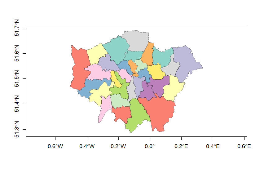
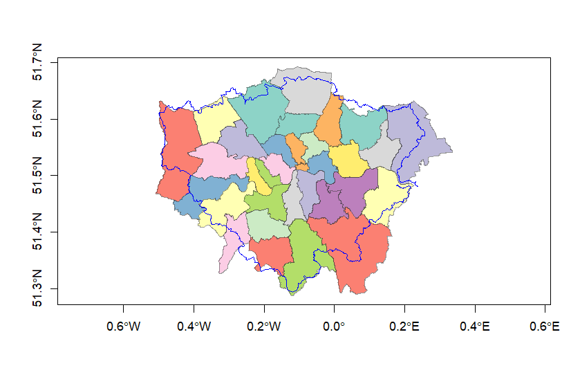
plot(st_geometry(london_poly), 
        col = sf.colors(length(london_poly$Name), 
                        categorical = TRUE), 
        axes=TRUE, border=grey(0.2, 0.5))

बिना रंग-भराव वाले मल्टी-पॉलीगॉन प्लॉट्स.

रंग-भराव वाले मल्टी-पॉलीगॉन प्लॉट्स.

plot() से लाइन्स प्लॉट करना

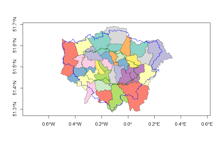
london_loop के लिए st_geometry() से पोलिलाइन्स बनाएँ
- add को TRUE करें
- col नीला करें
यही london_capital पर भी लागू करें

plot(st_geometry(london_loop),

        add=TRUE,

        col="blue")

plot(st_geometry(london_capital), 
        add=TRUE, 
        col="darkgreen")

एक गोल पथ वाला मानचित्र.

दो गोल पथों वाला मानचित्र.

plot() से पॉइंट्स प्लॉट करना

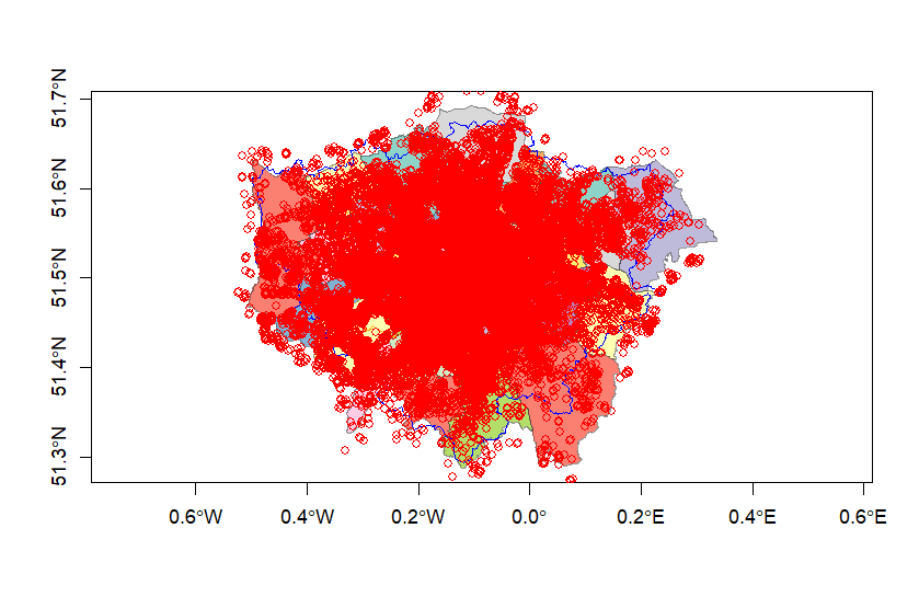
st_geometry() से पॉइंट्स जोड़ें
```
plot(st_geometry(listings_geo), add=TRUE, col='red')
```

sf पॉइंट्स प्लॉट करना.

ggplot() से पॉलीगॉन प्लॉट करना

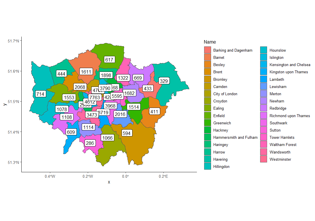
ggplot() से sf की लेयर्स प्लॉट कर सकते हैं
दो लेयर्स के लिए coordinate reference system (CRS) मिलाना आवश्यक है

ggplot से बना जियोस्पैशियल मैप.

num_listings <- listings %>% 
  group_by(neighbourhood) %>%
  summarize(`Number of listings` = n(),
            longitude = mean(longitude),
            latitude = mean(latitude),
            .groups = "drop") %>%

  st_as_sf(coords = c("longitude", "latitude"))

st_crs(num_listings) <- st_crs(london_poly)

ggplot_map <- ggplot(london_poly) + 
  geom_sf(aes(fill = Name)) +

  geom_sf_label(data=num_listings, 
              aes(label=`Number of listings`)) +
  theme_classic()

अभ्यास करते हैं!

shinydashboard के साथ डैशबोर्ड बनाना