डेटा का मॉडल

R में limma के साथ Differential Expression Analysis

John Blischak

Instructor

विश्लेषण के लिए तैयार

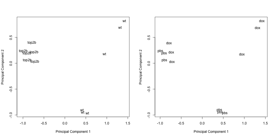
# Plot principal components labeled by genotype
plotMDS(eset, labels = pData(eset)[, "genotype"], gene.selection = "common")
# Plot principal components labeled by treatment
plotMDS(eset, labels = pData(eset)[, "treatment"], gene.selection = "common")

डिफरेंशियल एक्सप्रेशन एनालिसिस के स्टेप्स

model.matrix से डिज़ाइन मैट्रिक्स बनाएँ
makeContrasts से कॉन्ट्रास्ट्स मैट्रिक्स बनाएँ
lmFit, contrasts.fit, और eBayes से कॉन्ट्रास्ट्स टेस्ट करें

डॉक्सोरूबिसिन स्टडी के लिए ग्रुप-मीन्स मॉडल

$$ Y = \beta_1 X_1 + \beta_2 X_2 + \beta_3 X_3 + \beta_4 X_4 + \epsilon $$

$\beta_1$ - dox से ट्रीट किए गए top2b चूहों में औसत एक्सप्रेशन स्तर
$\beta_2$ - pbs से ट्रीट किए गए top2b में औसत एक्सप्रेशन स्तर
$\beta_3$ - dox से ट्रीट किए गए wt चूहों में औसत एक्सप्रेशन स्तर
$\beta_4$ - pbs से ट्रीट किए गए wt चूहों में औसत एक्सप्रेशन स्तर

डॉक्सोरूबिसिन स्टडी के लिए कॉन्ट्रास्ट्स

	$\beta_1$	$\beta_2$	$\beta_3$	$\beta_4$
`genotype`	top2b	top2b	wt	wt
`treatment`	dox	pbs	dox	pbs

Response of wild type mice to dox treatment: $\beta_3 - \beta_4 = 0$
Response of Top2b null mice to dox treatment: $\beta_1 - \beta_2 = 0$
Differences between Top2b null and wild type mice in response to dox treatment: $(\beta_1 - \beta_2) - (\beta_3 - \beta_4) = 0$

डॉक्सोरूबिसिन स्टडी की टेस्टिंग

lmFit से मॉडल कोएफिशिएंट्स फिट करें
contrasts.fit से कॉन्ट्रास्ट्स फिट करें
eBayes से t-स्टैटिस्टिक्स निकालें

# Summarize results
results <- decideTests(fit2)
summary(results)

# Create a Venn diagram
vennDiagram(results)

अभ्यास करते हैं!

R में limma के साथ Differential Expression Analysis