Dimensionality घटाना

R में Feature Engineering

Jorge Zazueta

Research Professor and Head of the Modeling Group at the School of Economics, UASLP

Zero variance फीचर्स

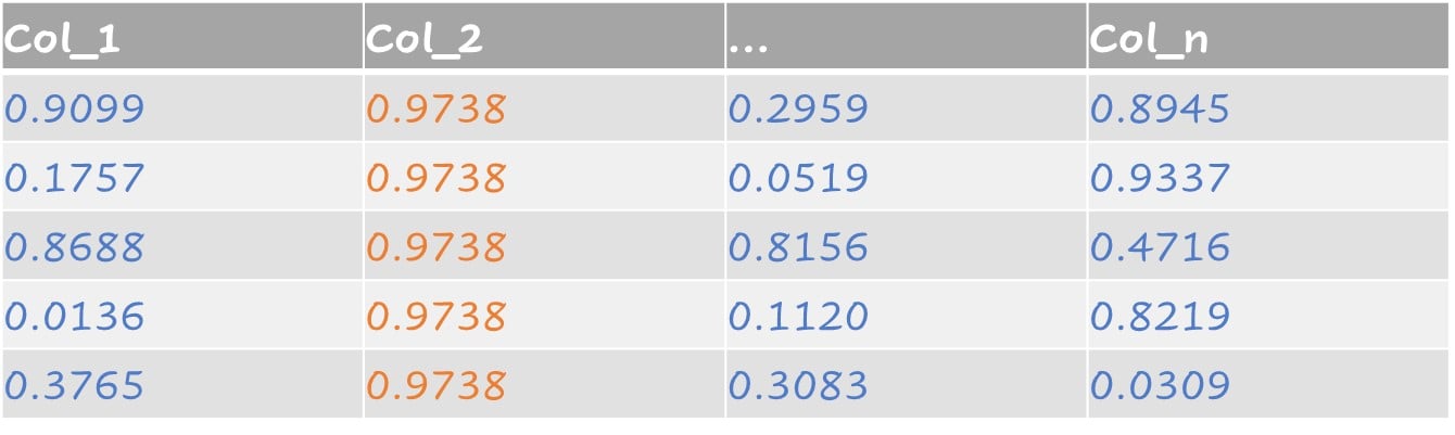
कुछ डेटासेट्स में ऐसे कॉलम होते हैं जिनकी वैल्यू स्थिर होती है या variance शून्य होता है. इन्हें फ़िल्टर करने के लिए recipe() में step_zv() जोड़ें.

शून्य variance वाले फीचर को दर्शाती तालिका.

Near-zero variance फीचर्स

Near-zero variance फीचर्स में वे प्रेडिक्टर्स शामिल हैं जिनकी वैल्यू एक ही हो, और वे जिनमें नीचे दोनों विशेषताएँ हों:

सैंपल्स की संख्या की तुलना में बहुत कम यूनिक वैल्यूज़
सबसे आम वैल्यू की फ़्रीक्वेंसी का दूसरी सबसे आम वैल्यू की फ़्रीक्वेंसी से अनुपात बड़ा हो

Near-zero variance का उदाहरण:

100 ऑब्ज़र्वेशन्स में दो अलग वैल्यू हैं, पर एक सिर्फ एक बार आती है.

step_nzv() ऐसे प्रेडिक्टर्स को पहचानकर हटाता है.

Principal Component Analysis (PCA)

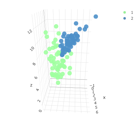
मूल तीन-डाइमेंशनल डेटासेट, दो क्लासेज के साथ.

दो डेटा क्लासेस वाला तीन-आयामी ग्राफ.

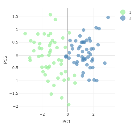
पहले दो principal components से रिप्रेज़ेंट किया गया घटाया हुआ डेटासेट.

पहले दो principal components के स्कैटरप्लॉट में दो डेटा क्लासेस दिखाता द्वि-आयामी ग्राफ.

चलो एक recipe प्रेप करें

PCA चलाने के लिए एक recipe बनाएँ और prep() से आउटपुट लें.

pc_recipe <- 
recipe(~., data = loans_num) %>%
  step_nzv(all_numeric()) %>%
  step_normalize(all_numeric()) %>%
  step_pca(all_numeric())

pca_output <- prep(pc_recipe)

उपलब्ध जानकारी देखने के लिए pca_output पर names() कॉल करें.

names(pca_output)

 [1] "var_info"       "term_info"     
 [3] "steps"          "template"      
 [5] "levels"         "retained"      
 [7] "requirements"   "tr_info"       
 [9] "orig_lvls"      "last_term_info"

Variance explained ढूँढना

pca_output ऑब्जेक्ट से standard deviation निकालें और variance explained निकालें.

stdv <- pca_output$steps[[3]]$res$sdev

var_explained <- stdv^2/sum(stdv^2)

PCA = tibble(PC = 1:length(stdv),
          var_explained = var_explained, 
          cumulative = cumsum(var_explained))

तालिका: प्रत्येक principal component द्वारा समझाया गया variance.

# A tibble: 5 × 3
     PC var_explained cumulative
  <int>         <dbl>      <dbl>
1     1        0.315       0.315
2     2        0.214       0.529
3     3        0.202       0.730
4     4        0.198       0.928
5     5        0.0722      1

Variance explained का विज़ुअलाइज़ेशन

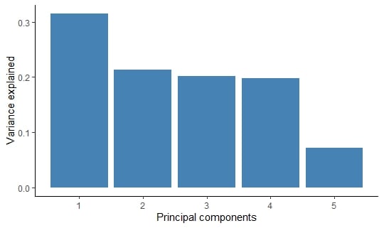
ggplot2 से आउटपुट को कॉलम चार्ट के रूप में प्लॉट कर सकते हैं.

PCA %>% 
ggplot(aes(x = PC, 
           y = var_explained)) +
  geom_col(fill = "steelblue") +
  xlab("Principal components") +
  ylab("Variance explained")

Principal component द्वारा समझाया गया variance.

Principal component द्वारा समझाया गया variance दिखाता कॉलम चार्ट.

अभ्यास करते हैं!

R में Feature Engineering