Posterior estimation & inference

RJAGS के साथ Bayesian Modeling

Alicia Johnson

Associate Professor, Macalester College

Bayesian regression मॉडल

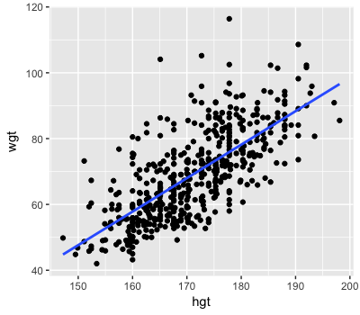
$Y_i$ = वयस्क $i$ का वज़न (kg)
$X_i$ = वयस्क $i$ की लंबाई (cm)

$\;$

मॉडल

$Y_i \sim N(m_i, s^2)$
$m_i = a + b X_i$

$a \sim N(0, 200^2)$
$b \sim N(1, 0.5^2)$
$s \sim \text{Unif}(0, 20)$

Posterior point estimation

summary(weight_sim_big)

1. Empirical mean and standard deviation for each variable,
   plus standard error of the mean:
      Mean      SD  Naive SE Time-series SE
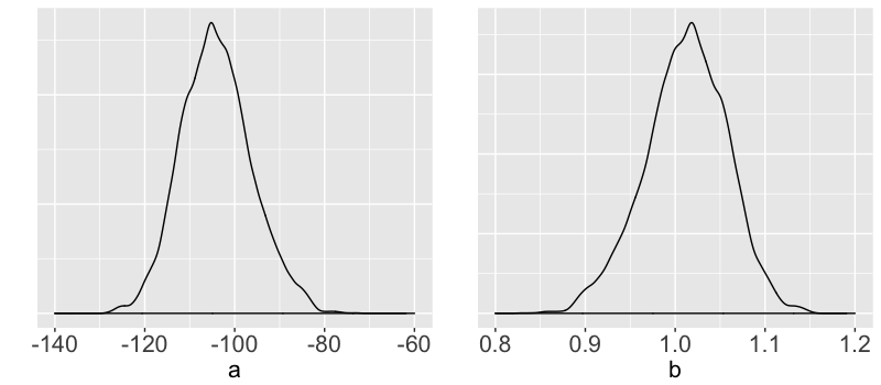
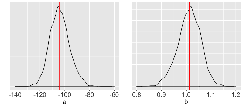
a -104.038 7.85296 0.0248332       0.661515
b    1.012 0.04581 0.0001449       0.003849
s    9.331 0.29495 0.0009327       0.001216

2. Quantiles for each variable:
       2.5%       25%      50%     75%   97.5%
a -118.6843 -109.5171 -104.365 -99.036 -87.470
b    0.9152    0.9828    1.014   1.044   1.098
s    8.7764    9.1284    9.322   9.524   9.933

$a$ का posterior mean $\approx$ -104.038

$b$ का posterior mean $\approx$ 1.012

Posterior point estimation

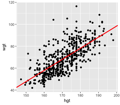
Posterior mean ट्रेंड:

$m_i = -104.038 + 1.012 X_i$

Markov chain आउटपुट:

head(weight_chains)

             a        b        s
[1,] -113.9029 1.072505 8.772007
[2,] -115.0644 1.077914 8.986393
[3,] -114.6958 1.077130 9.679812
[4,] -115.0568 1.072668 8.814403
[5,] -114.0782 1.071775 8.895299
[6,] -114.3271 1.069477 9.016185

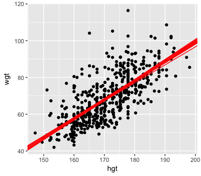
Posterior अनिश्चितता

Posterior mean ट्रेंड:

$m_i = -104.038 + 1.012 X_i$

Markov chain आउटपुट:

head(weight_chains)

             a        b        s
[1,] -113.9029 1.072505 8.772007
[2,] -115.0644 1.077914 8.986393
[3,] -114.6958 1.077130 9.679812
[4,] -115.0568 1.072668 8.814403
[5,] -114.0782 1.071775 8.895299
[6,] -114.3271 1.069477 9.016185

Posterior credible intervals

summary(weight_sim_big)

1. Empirical mean and standard deviation for each variable,
   plus standard error of the mean:
      Mean      SD  Naive SE Time-series SE
a -104.038 7.85296 0.0248332       0.661515
b    1.012 0.04581 0.0001449       0.003849
s    9.331 0.29495 0.0009327       0.001216

2. Quantiles for each variable:
       2.5%       25%      50%     75%   97.5%
a -118.6843 -109.5171 -104.365 -99.036 -87.470
b    0.9152    0.9828    1.014   1.044   1.098
s    8.7764    9.1284    9.322   9.524   9.933

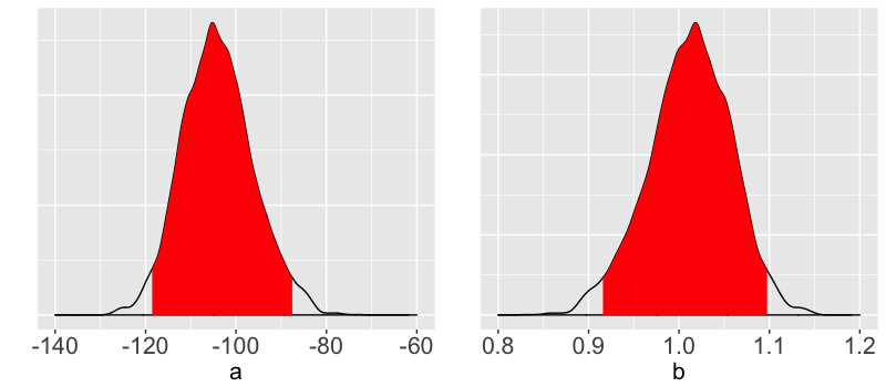
$a$ के लिए 95% posterior credible interval: (-118.6843, -87.470)

$b$ के लिए 95% posterior credible interval: (0.9152, 1.098)

Posterior credible intervals

Interpretation

हमारे priors और observed डेटा के आधार पर, 95% (posterior) संभावना है कि $b$ 0.9152 और 1.098 kg/cm के बीच है.

Posterior probabilities

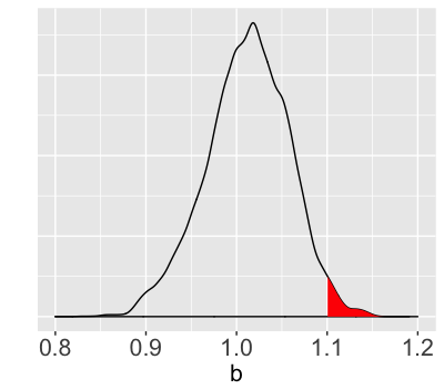
table(weight_chains$b > 1.1)

FALSE  TRUE 
97835  2165

mean(weight_chains$b > 1.1)

0.02165

Interpretation:
$b$ के 1.1 kg/cm से अधिक होने की posterior संभावना 2.165% है.

अभ्यास करते हैं!

RJAGS के साथ Bayesian Modeling