สเปกโตรแกรม — การเปลี่ยนแปลงเชิงสเปกตรัมของเสียงตามเวลา

Machine Learning สำหรับข้อมูล Time Series ใน Python

Chris Holdgraf

Fellow, Berkeley Institute for Data Science

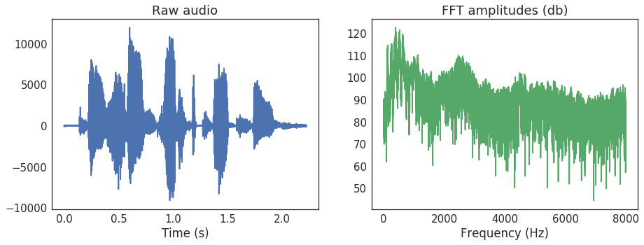
Fourier transforms

ข้อมูล timeseries ประกอบด้วยองค์ประกอบที่เปลี่ยนแปลงเร็วและช้าผสมกัน
ในแต่ละช่วงเวลา เราสามารถอธิบายสัดส่วนของทั้งสองส่วนได้
วิธีที่ง่ายที่สุดคือ Fourier Transform
เทคนิคนี้แปลง timeseries เป็น array ที่แสดงถึงการรวมกันของการสั่นสะเทือนต่าง ๆ

Fourier Transform (FFT)

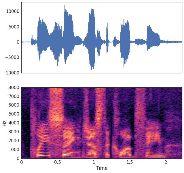
สเปกโตรแกรม: การรวม Fourier transforms แบบ windowed

สเปกโตรแกรมคือชุด Fourier transforms แบบ windowed ที่คำนวณต่อเนื่องตามเวลา
คล้ายกับการคำนวณค่าเฉลี่ยแบบ rolling:
1. กำหนดขนาดและรูปร่างของ window
2. ณ จุดเวลาหนึ่ง คำนวณ FFT สำหรับ window นั้น
3. เลื่อน window ไปทีละหนึ่งช่วง
4. รวมผลลัพธ์ที่ได้
เรียกว่า Short-Time Fourier Transform (STFT)

การคำนวณ STFT

คำนวณ STFT ได้ด้วย librosa
มีพารามิเตอร์หลายตัวที่ปรับได้ เช่น ขนาด window
เราจะแปลงค่าเป็น เดซิเบล เพื่อทำให้ค่าเฉลี่ยของทุกความถี่อยู่ในระดับเดียวกัน
จากนั้นแสดงผลด้วยฟังก์ชัน specshow()

การคำนวณ STFT ด้วยโค้ด

# Import the functions we'll use for the STFT
from librosa.core import stft, amplitude_to_db
from librosa.display import specshow
import matplotlib.pyplot as plt

# Calculate our STFT
HOP_LENGTH = 2**4
SIZE_WINDOW = 2**7
audio_spec = stft(audio, hop_length=HOP_LENGTH, n_fft=SIZE_WINDOW)

# Convert into decibels for visualization
spec_db = amplitude_to_db(audio_spec)

# Visualize
fig, ax = plt.subplots()
specshow(spec_db, sr=sfreq, x_axis='time', 
         y_axis='hz', hop_length=HOP_LENGTH, ax=ax)

การสร้างฟีเจอร์เชิงสเปกตรัม

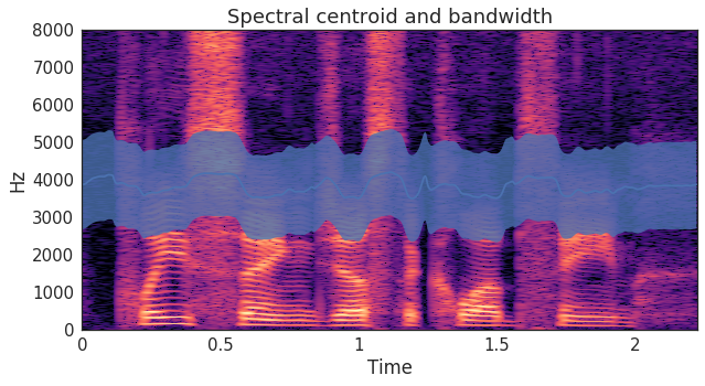
แต่ละ timeseries มีรูปแบบเชิงสเปกตรัมที่แตกต่างกัน
วิเคราะห์สเปกโตรแกรมเพื่อหารูปแบบเหล่านี้ได้
ตัวอย่างเช่น spectral bandwidth และ spectral centroids แสดงให้เห็นว่าพลังงานส่วนใหญ่อยู่ที่ใดในแต่ละช่วงเวลา

การคำนวณฟีเจอร์เชิงสเปกตรัม

# Calculate the spectral centroid and bandwidth for the spectrogram
bandwidths = lr.feature.spectral_bandwidth(S=spec)[0]
centroids = lr.feature.spectral_centroid(S=spec)[0]

# Display these features on top of the spectrogram
fig, ax = plt.subplots()
specshow(spec, x_axis='time', y_axis='hz', hop_length=HOP_LENGTH, ax=ax)
ax.plot(times_spec, centroids)
ax.fill_between(times_spec, centroids - bandwidths / 2, 
                centroids + bandwidths / 2, alpha=0.5)

การรวมฟีเจอร์เชิงสเปกตรัมและเวลาใน classifier

centroids_all = []
bandwidths_all = []
for spec in spectrograms:
    bandwidths = lr.feature.spectral_bandwidth(S=lr.db_to_amplitude(spec))
    centroids = lr.feature.spectral_centroid(S=lr.db_to_amplitude(spec))
    # Calculate the mean spectral bandwidth
    bandwidths_all.append(np.mean(bandwidths))  
    # Calculate the mean spectral centroid
    centroids_all.append(np.mean(centroids))  

# Create our X matrix
X = np.column_stack([means, stds, maxs, tempo_mean, 
                     tempo_max, tempo_std, bandwidths_all, centroids_all])

มาฝึกกันเถอะ!

Machine Learning สำหรับข้อมูล Time Series ใน Python