Autocorrelation

การวิเคราะห์อนุกรมเวลาใน R

David S. Matteson

Associate Professor at Cornell University

Autocorrelation - I

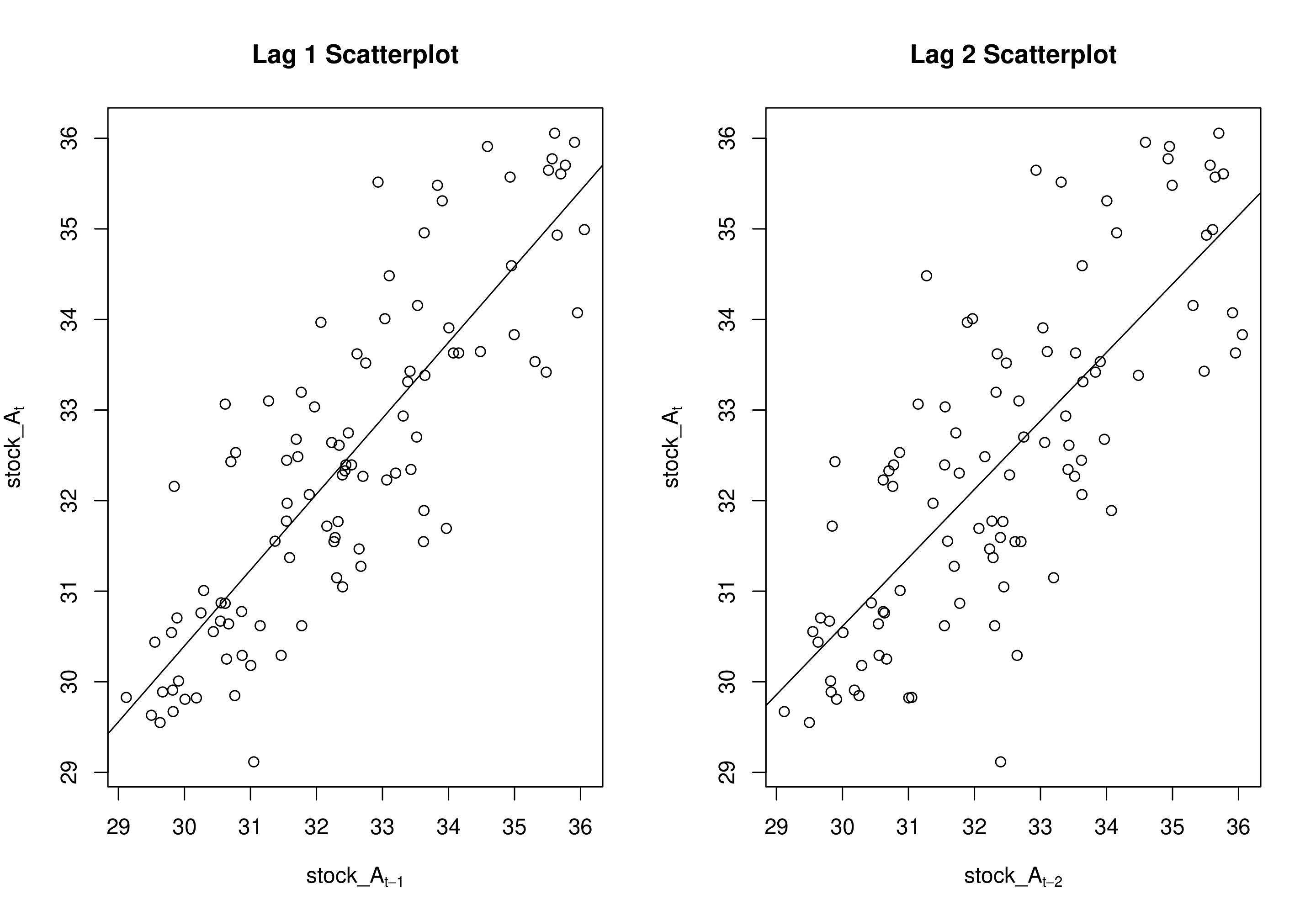
# Lag 1 Autocorrelation: 
# Correlation of stock A "today" and stock A "yesterday"
cor(stock_A[-100], stock_A[-1])

0.84

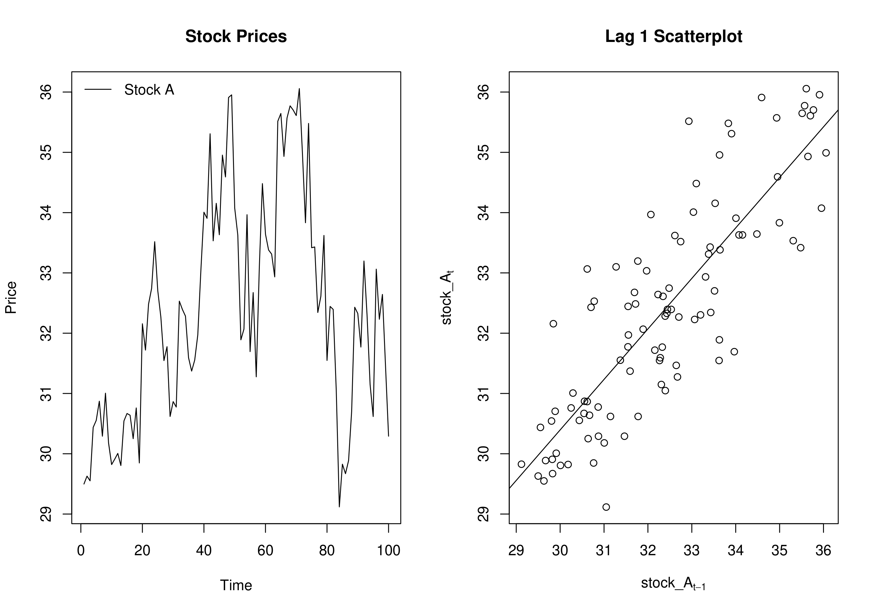
# Lag 2 Autocorrelation:
# Correlation of Stock A "today" and stock A "Two Days Earlier"
cor(stock_A[-(99:100)],stock_A[-(1:2)])

0.76

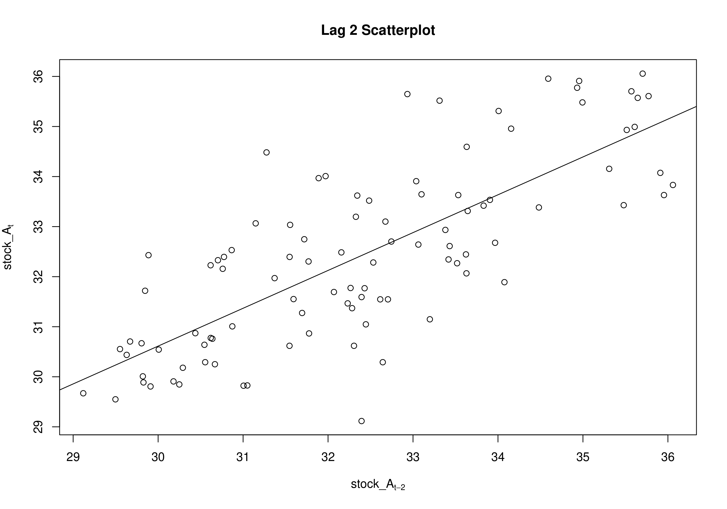
cor(stock_A[-100],stock_A[-1])

0.84

cor(stock_A[-(99:100)],stock_A[-(1:2)])

0.76

acf(stock_A, lag.max = 2, plot = FALSE)

Autocorrelations of series 'stock_A', by lag
  1    2
0.84  0.76

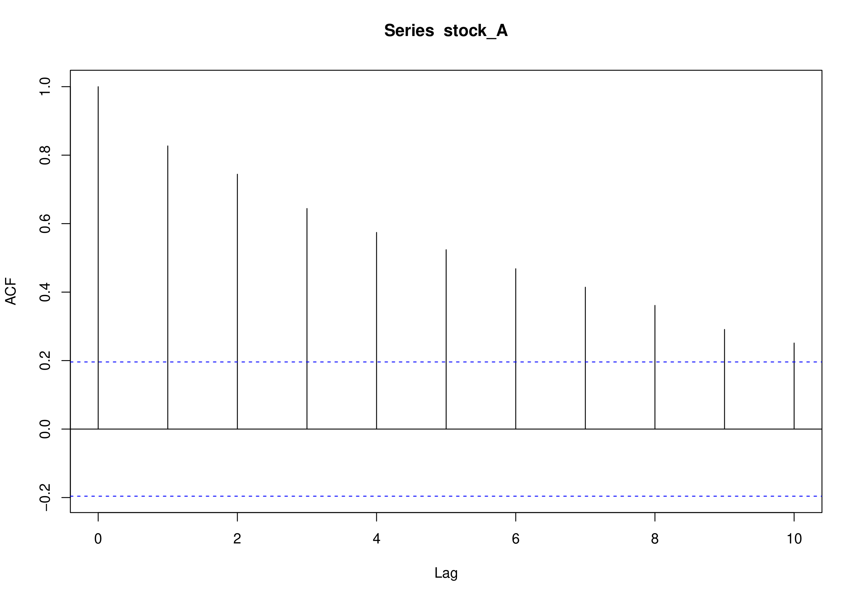
# Autocorrelation by lag: "The Autocorrelation Function" 
(ACF)acf(stock_A, plot = FALSE)

Autocorrelations of series 'stock_A', by lag
  1    2    3    4    5    6    7    8    9   10
0.84 0.76 0.64 0.57 0.52 0.46 0.41 0.36 0.29 0.25

acf(stock_A, plot = TRUE)

การวิเคราะห์อนุกรมเวลาใน R