Dynamisk harmonisk regression
Prognoser i R

Rob J. Hyndman
Professor of Statistics at Monash University
Dynamisk harmonisk regression

Dynamisk harmonisk regression
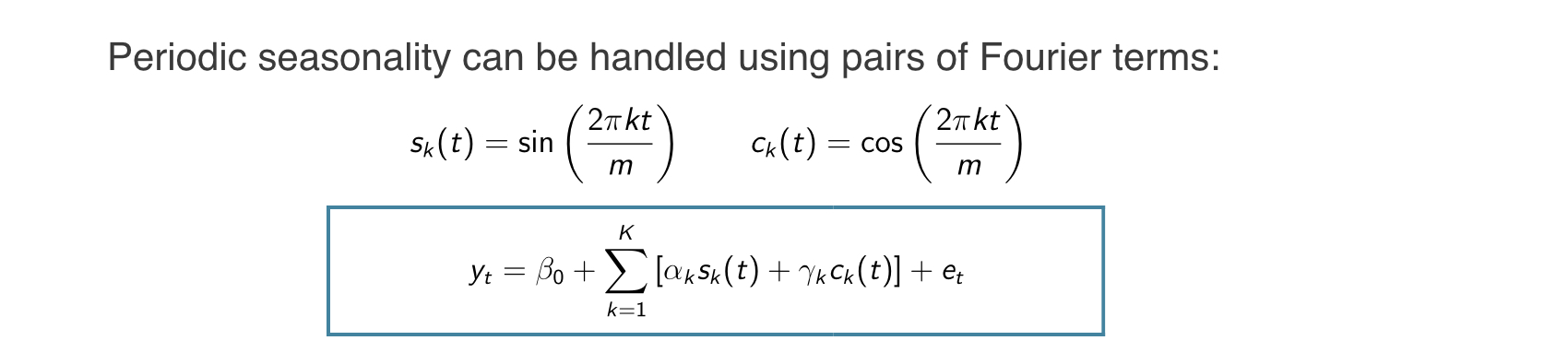
$m =$ säsongperiod
Varje periodisk funktion kan approximeras med summor av sin- och cos-termer för tillräckligt stort K
Regressionskoefficienter: $\alpha_k$ och $\gamma_k$
$e_t$ kan modelleras som en icke-säsongsmässig ARIMA-process
Förutsätter att säsongsmönstret är konstant
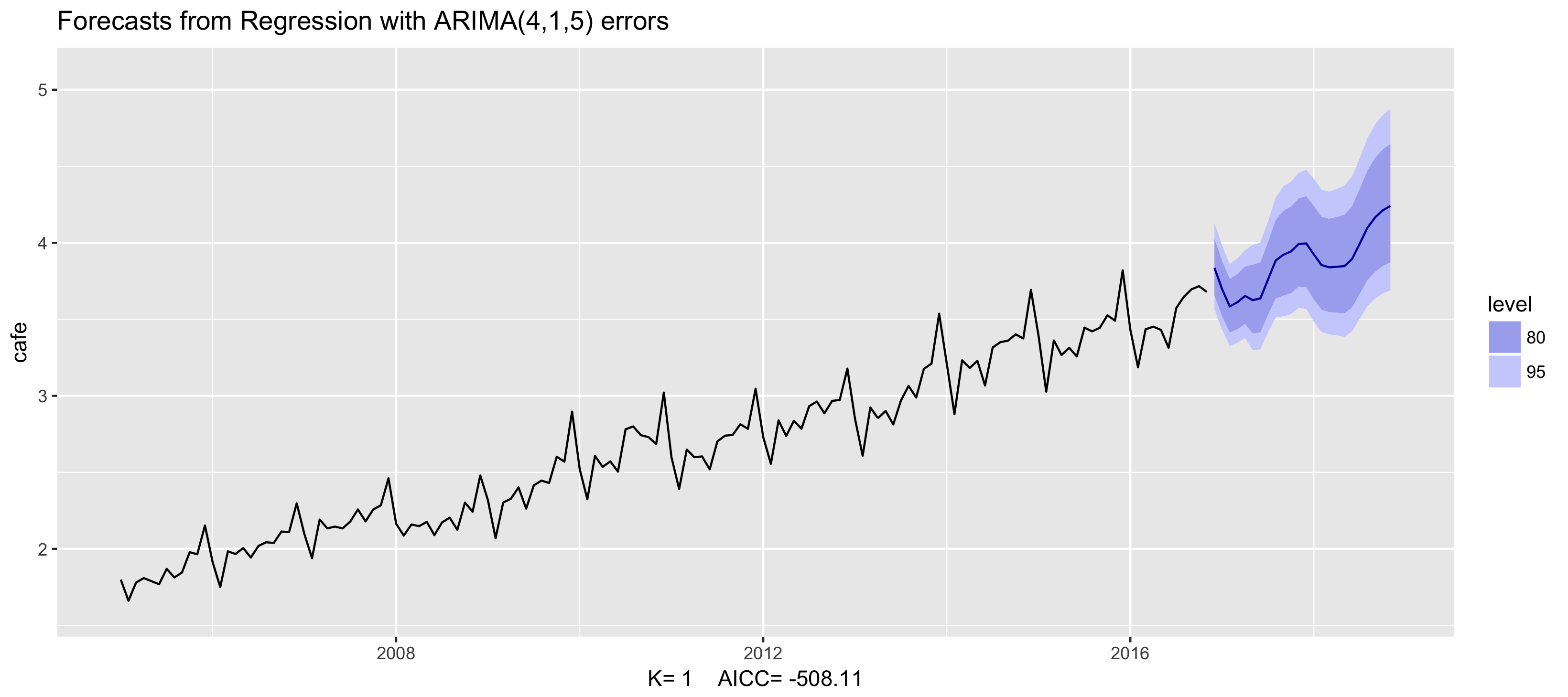
Exempel: Australiensiska caféutgifter
fit <- auto.arima(cafe, xreg = fourier(cafe, K = 1),
                  seasonal = FALSE, lambda = 0)
fit %>% forecast(xreg = fourier(cafe, K = 1, h = 24)) %>%
   autoplot() + ylim(1.6, 5.1)
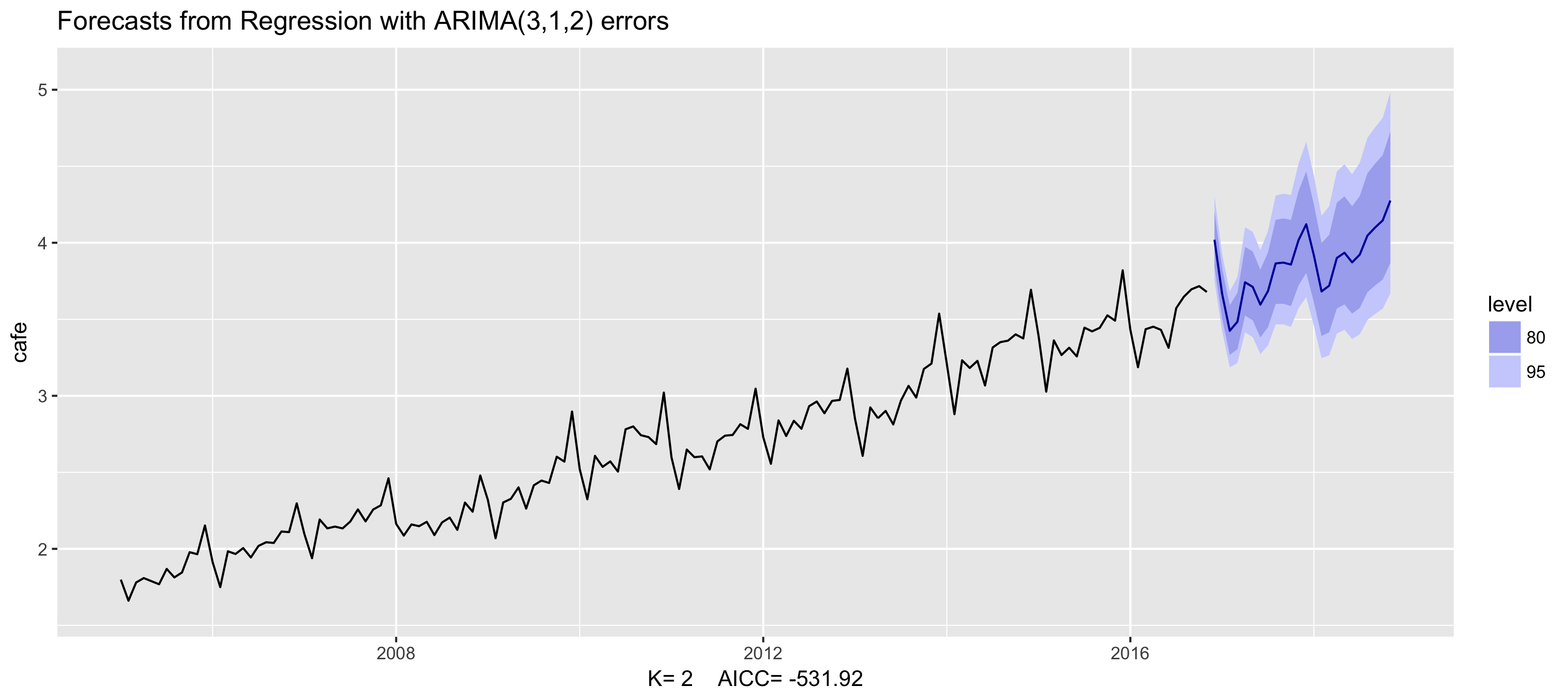
Exempel: Australiensiska caféutgifter
fit <- auto.arima(cafe, xreg = fourier(cafe, K = 2),
                  seasonal = FALSE, lambda = 0)
fit %>% forecast(xreg = fourier(cafe, K = 2, h = 24)) %>%
   autoplot() + ylim(1.6, 5.1)
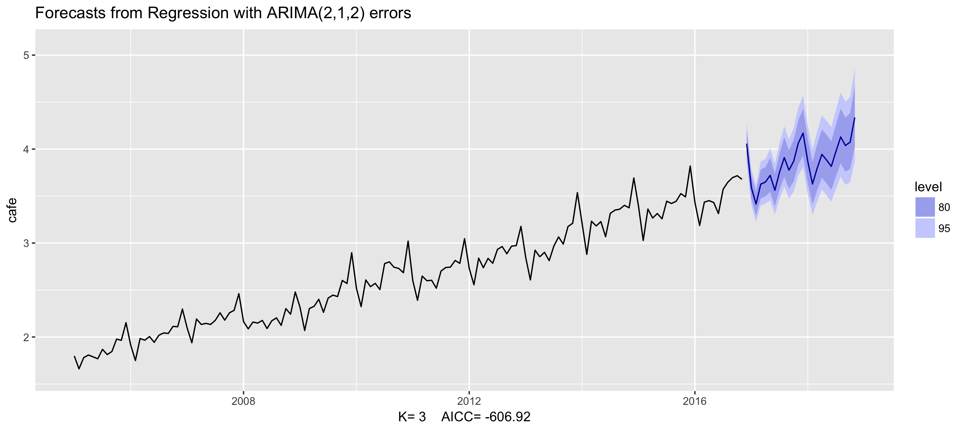
Exempel: Australiensiska caféutgifter
fit <- auto.arima(cafe, xreg = fourier(cafe, K = 3),
                  seasonal = FALSE, lambda = 0)
fit %>% forecast(xreg = fourier(cafe, K = 3, h = 24)) %>%
   autoplot() + ylim(1.6, 5.1)
Exempel: Australiensiska caféutgifter
fit <- auto.arima(cafe, xreg = fourier(cafe, K = 4),
                  seasonal = FALSE, lambda = 0)
fit %>% forecast(xreg = fourier(cafe, K = 4, h = 24)) %>%
   autoplot() + ylim(1.6, 5.1)
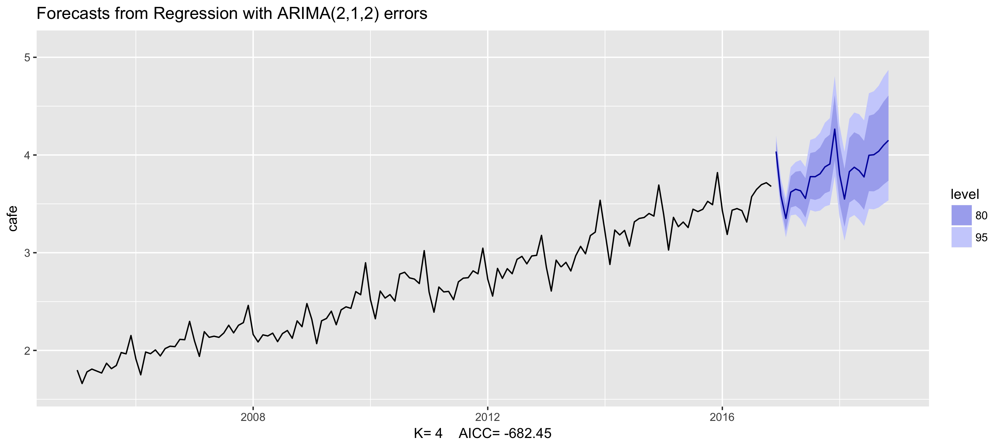
Exempel: Australiensiska caféutgifter
fit <- auto.arima(cafe, xreg = fourier(cafe, K = 5),
                  seasonal = FALSE, lambda = 0)
fit %>% forecast(xreg = fourier(cafe, K = 5, h = 24)) %>%
   autoplot() + ylim(1.6, 5.1)
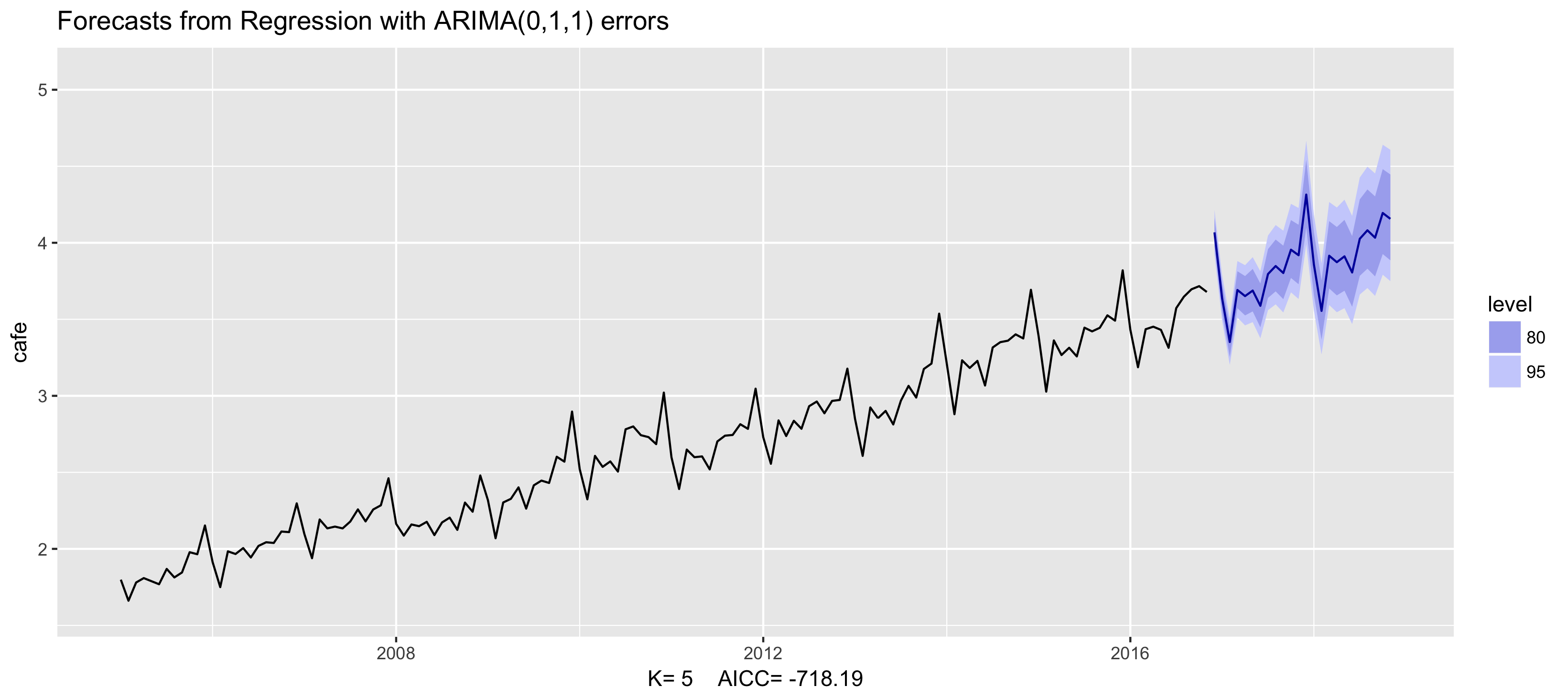
Exempel: Australiensiska caféutgifter
fit <- auto.arima(cafe, xreg = fourier(cafe, K = 6),
                  seasonal = FALSE, lambda = 0)
fit %>% forecast(xreg = fourier(cafe, K = 6, h = 24)) %>%
   autoplot() + ylim(1.6, 5.1)
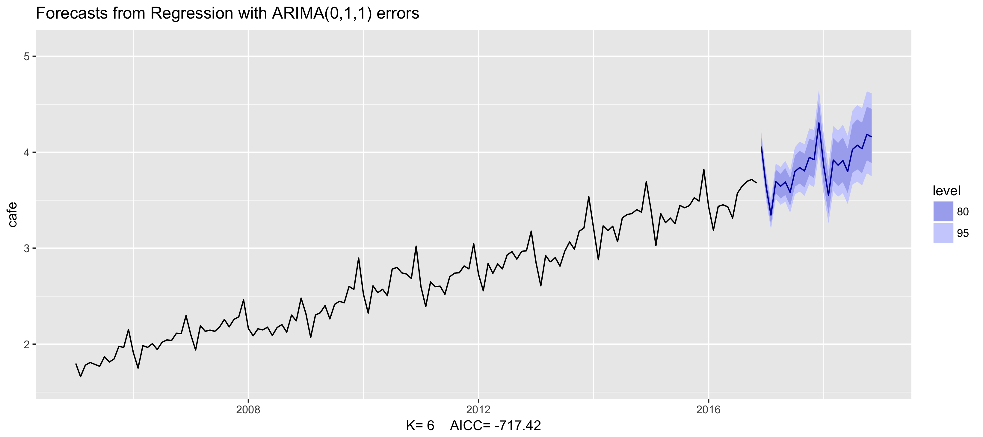
Dynamisk harmonisk regression

- Andra prediktorvariabler kan också läggas till: $x_{t,1},...,x_{t,r}$
- Välj K för att minimera $AIC_c$
- K kan inte vara mer än m/2
- Särskilt användbart för veckodata, dagsdata och data med kortare intervall.

